
J. Cent. South Univ. (2016) 23: 3018-3027
DOI: 10.1007/s11771-016-3365-9

Installation position determination of wind speed sensors on steel pole along a high-speed railway
XIONG Xiao-hui(��С��)1, 2, LIANG Xi-feng(��ϰ��)1, 2
1. Key Laboratory of Traffic Safety on Track of Ministry of Education, Changsha 410075, China;
2. School of Traffic & Transportation Engineering, Central South University, Changsha 410075, China
 Central South University Press and Springer-Verlag Berlin Heidelberg 2016
Abstract:
In order to consider the influence of steel pole on the measurement of wind speed sensors and determinate the installation position of wind speed sensors, the flow field around wind speed sensors was investigated. Based on the three-dimensional steady Reynolds-averaged Navier-Stokes equations and k-�� double equations turbulent model, the field flow around the wind speed sensor and the steel pole along a high-speed railway was simulated on an unstructured grid. The grid-independent validation was conducted and the accuracy of the present numerical simulation method was validated by experiments and simulations carried out by previous researchers. Results show that the steel pole has a significant influence on the measurement results of wind speed sensors. As the distance between two wind speed sensors is varied from 0.3 to 1.0 m, the impact angles are less than ��20��, it is proposed that the distance between two wind speed sensors is 0.8 m at least, and the interval between wind speed sensors and the steel pole is more than 1.0 m with the sensors located on the upstream side.
Key words:
high-speed railway; wind speed sensor; steel pole; numerical simulation; flow field��
1 Introduction
Under strong winds, aerodynamic loads would have a great effect on the operation safety of high-speed trains with an increasing risk of overturning [1-13]. Nowadays, cross wind effects on trains have become a common matter in daily life. Many scholars and institutes with developed railway traffic and transportation in their countries have carried out lots of research and obtained large practical achievements to prevent train accidents [2, 14-18]. One of these effective measurements is to carry out the regulation of train operation, and establish a strong winds early warning system (SWEWS).
For the SWEWS, the countries in wind regions have respectively built ones which are more suitable for their own national conditions [2, 19-21]. In Japan, the WINDAS system was invented to improve the transportation efficiency of railways at crosswind conditions with thousands of anemometers installed along railway lines in 2001 [22]. In Korea, the wind monitoring system consists of wind speed sensors and direction sensors. The speed sensors are used cup anemometers with the measure range of 0-75 m/s, while the directional ones are the blade type. It is also suggested that the distance between the wind monitoring system and the nearest obstacle should be 10 times the height of the obstacle. If not, the reliability of wind sensors would be influenced, which can lead to getting inaccurate information. Thus, the system is usually located on the top of an iron tower which is away from the railway line [21]. In Germany, Deutsche Bahn AG (German Rail) developed a wind warning system to protect high-speed trains against strong crosswinds in 1998. Within this so-called Nowcasting System, a short-term prediction of the maximum wind speed is made on the basis of continuous wind measurements at distinct locations of a high-speed railway line [20]. And every monitoring point has two 3-D ultrasonic anemometers which are 4 m above the rail level and at a distance of 4 m from the center line of the nearer track. France also has its own Vigilance System. Taking the wind monitoring system along Mediterranean high-speed railway line for example, the mechanical propeller anemometers are installed on two independent dismountable masts which are 5 m in high. Its distances above the rail level and away from the center line of the nearer track are all 4 m [21]. In China, the systems have been built along Lanzhou-Xinjiang railway, Qinghai- Tibet railway and high-speed railways which are easily affected by strong winds/monsoons [19, 23-25]. Along Lanzhou-Xinjiang and Qinghai-Tibet railways, the wind speed monitoring stations are generally set up upstream of the railway line where the wind speed can respond to the incoming flow [24-25]. But taking the distance between the station and the train into account, the measurement by the sensor can��t reflect the wind velocity around the railway line at the same time. Therefore, along high-speed railways constructed, the sensors are often installed in a horizontal holder which is fixed on the steel pole and located 4 m above the rail level. Every monitoring point has two sensors as in some other countries. They are outwards and their line of centers is paralleled to the railway line. The sensor models are used the Lambrecht hot-zone from Germany and the Vaisala ultrasonic from Finland. Every monitoring point installs two sensors with a combination of a hot-zone and an ultrasonic, or just two ultrasonic models. However, the cross-section of a steel pole is so large that the airflow would be blocked by the steel pole, when the crosswind is along the incoming flow. Then, the sensors may be in a deceleration zone. The measurement data would be influenced by the steel pole. While the sensors are near the sides of the pole and the effects tend to be more. However, when the crosswind direction is opposite, for the shielding effect of the steel pole, the sensors may be in an acceleration or deceleration zone, and then the measurement results would be doubtful and mistake. Thus, for the layout mentioned along China high-speed railways, it needs to carry out further investigations.
2 Numerical method
Figure 1 is the installment photos of the wind sensors on the steel pole at the high-speed railway line in China. When the wind speed reaches above 30 m/s, the high-speed trains are forbidden to run into gale regions, and thus the wind speed in the current paper is 30 m/s (Based on Article 170 of the ��Interim Measures for the Management of Beijing�CTianjin Intercity Railway (TG-QT106��2008)��). Then, the air can be considered to be incompressible. The maximal diameter D of the Lambrecht hot-zone from Germany is 105 mm, while the cross-section of a steel pole is 300 mm��300 mm. At the ambient temperature with a standard atmospheric pressure, the air kinematic viscosity ��=1.46��10-5 m2/s, and the Reynolds number of the sensor, Re=VD/��= 2.16��105 >> Rec, where, Rec equal to 2320 is the critical Reynolds number for the laminar and turbulent flow. Therefore, the 3-D, steady N-S equation and k-�� double equations turbulent model represents the most extensive method in engineering application [12, 16] to compute the flow field around the steel pole.

Fig. 1 Installment of wind sensors on steel pole
In general, the equations are reduced to the following form.
Continuity:
 (1)
(1)
Momentum:
 (2)
(2)
where ui, p and �� are the mean velocity vector, mean static pressure and constant air density, respectively; �� is the dynamic viscosity of air; The eddy viscosity ��t is related to turbulent kinetic energy k and its rate of dissipation �� by the following relation when the k-�� model is used to close the above set of equations:
 (3)
(3)
where C�� is a turbulent constant; k and �� are obtained from the standard k-�� turbulence model equations which can be expressed as follows:
Turbulence kinetic energy k:
 (4)
(4)
Dissipation rate ��:

 (5)
(5)
Constant coefficients:
C��=0.09, C1��=1.44, C2��=1.92, ��k=1.0, ����=1.3 (6)
In the current simulation, the pressure-based solver used the SIMPLEC algorithm to introduce pressure into the continuity equation. A second-order upwind scheme was chosen for solving the Navier�CStokes equations. For the residual of continuity, the absolute criterion of convergence was set to 10-7 with over 6500 iterations. During the calculations, wind speeds around the pole are monitored for judging the convergence of the solution.
3 Geometry description and wind direction definition
For the Lambrecht hot-zone from Germany and the Vaisala ultrasonic from Finland are similar in the dimensions. The Lambrecht is chosen for the research on the interaction disturbance of the flow field due to the sensors themselves. Its maximal diameter D is 105 mm with the length l of 311 mm, as shown in Fig. 2(a). The model of a steel pole is the double H type, of which cross-section is 300 mm��300 mm, as demonstrated in Fig. 2(b).
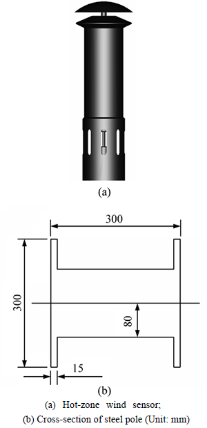
Fig. 2 Computational models:
In this simulation, when a wind speed sensor is installed on the steel pole, to guarantee the measurement accuracy of the sensor, it should be taken the wind direction into account. The wind direction definition is illustrated in Fig. 3, and it represents the included angle between the wind and the positive direction of the y axis. Considered the effect of wind directions as much as possible, it is chosen as 0��, 15��, 30��, 45��, 60��, 75�� and 90��, respectively. When ��=0��, the incoming flow is parallel with the railway line. When ��=90��, the incoming flow is normal to the railway line. For the symmetry structure of the steel pole, as the direction varies from 0�� to -90��, we can refer to the velocity distribution between the 0�� and 90��. Under this condition, two virtual points representing the sensors are set up on the downstream side of the steel pole to obtain the wind speed. The distance between the two sensors is defined as h, and the distance of their center line away from the center of the pole cross-section is specified as d.
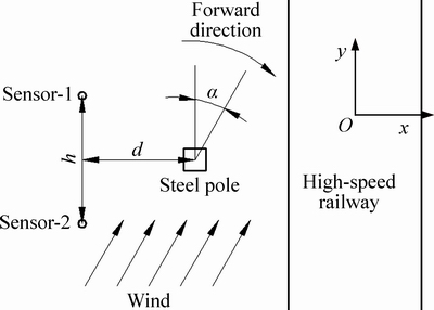
Fig. 3 Wind direction definition
4 Computational domain and boundary conditions
In China, the steel pole along a high-speed railway is an upright structure with a fixed cross-section, and the effect of the ground on the flow around the pole is much weaker at a certain height, thus the computational domain can be demonstrated in Fig. 4. The coordinate system is also defined as shown in Fig. 4. The characteristic length is the width of the pole and is denoted by L. And a prism layer of 10 cells is created in a belt around the pole. The thickness of the first layer is 1.75 mm to ensure the use of wall function in k-epsilon turbulence model. When the flow field around a sensor is investigated, the pole in the computational domain will be replaced by the sensor which will be laid at the coordinate origin.
In Fig. 4, the surface of the pole or the sensor is set as no slip wall. Inlet-1 and Inlet-2 are treated as velocity-inlet with the velocity components of the x and y axes, respectively. The resultant velocity of the two is 30 m/s. At the outlet, a pressure value 0 is adopted. At the top and bottom of the computational domain, the symmetry is set.
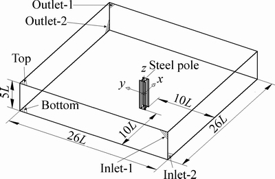
Fig. 4 Computational domain
5 Results and discussion
5.1 Assessment of numerical accuracy for simulation
To determine the effect of mesh resolution on the results, several simulations were conducted at three different meshes with different numbers of cells: coarse, medium and fine meshes consisting of 3.25��106, 4.26��106 and 5.29��106 cells, respectively, and the results were compared. In simulations, the wind direction is 90�� with a speed of 30 m/s. The velocity ratio RU of the horizontal plane at x=1.0 m is studied as illustrated in Fig. 5. The velocity ratio RU is defined as follows:
RU=Uxy/U (7)
where Uxy is the wind speed of this point in the xy horizontal plane; U is the incoming flow speed.

Fig. 5 Velocity ratio RU
The results of three different meshes closely fit together, which indicates that the coarse mesh is adequate and can be used for the follow-up research. Figure 6 shows the coarse mesh of the cross-section of the pole.
In order to validate the accuracy of the present numerical method, Fig. 7 shows the validation result obtained using this program with the centre line velocity in front of the square. The experimental data are from Ref. [26]. and the numerical simulation data are from Ref. [27]. Compared with the recorded values, Fig. 7 presents reasonable agreement with the experimental and simulation results.
5.2 Flow field around sensor
Along railway lines, to guarantee the accuracy of measured data, there are always two wind speed sensors installed at a monitor point. According to the flow theory of a bluff body, if the wind direction is parallel with the connected line of two sensors and the latter sensor will be influenced by the former one. Thus, it needs to study the flow field around a sensor. In simulations, only one sensor is located in the computational zone, while the other is a virtual sensor instead (According to the principle of measurement by the hot-zone wind speed sensor, the data obtained are relative to their constant coefficients, convective heat transfer coefficient, passing electric current value, and so on. When these parameters are unknown, the velocity around the sensor in the simulation cannot be used to reflect the speed of the far-field airflow. So, in order to eliminate the disturbance of the flow field due to the sensors themselves, the method of setting up a virtual point and reading its speed value is chosen).

Fig. 6 Mesh distribution of cross-section

Fig. 7 Comparison with numerical and experimental results
To obtain a comprehensive analysis, the flow field around the wind speed sensor, different radial cylindrical surfaces have been drawn, as shown in Fig. 8(a). The radius is defined as R and is chosen as 0.3, 0.5, 0.8 and 1.0 m, respectively. Figure 8(b) shows the streamlines around the wind speed sensor. It can be discovered that there is a region with larger velocity variation, which means that the speed tends to reduce at the upstream side of the sensor. Subsequently, the flow accelerates bypass it, and slows down behind the sensor to a large extent. For the sensor isn��t the regular cylinder, the velocity around it will be a little different, as demonstrated in Fig. 8(c). Behind the sensor, there is a region with low speed and a peak value of the wind speed, which is close to the lower part. Except in this region, the speeds meet the allowable measured deviations of 10% based on the in-coming flow speed all not less than 30 m/s, but not more than 30.5 m/s. To find out the angle of influence at different distance between the sensor and the virtual one, allowable measured deviations of ��5% and ��10% are taken into consideration, and the contour lines of 27.0, 28.5 and 30 m/s are presented on the cylindrical surface in Fig. 8(c). For each contour line, there will be two peak values, a maximum and a minimum along the y axis. After that, two lines are drawn to connect the center line of the sensor with the peak values in the xy horizontal plane, as illustrated in Fig. 8(c). As a result, an angle �� which represents the largest region of influence at this cylindrical surface is coming into being. Based on this method, the angles of influence at different radial cylindrical surfaces can be found, as listed in Table 1.
It is discovered that as the distance is varied from 0.3 m to 1.0 m, the most adverse angles are not in excess of ��20�� (40��). The closer the distance, the larger the angle of influence. At the distance of 0.3 m, with an allowable deviation of 5%, the angle of impact is 39.3��. While at the distance of 1.0 m, it is 15.5��. If the deviation is increased to 10%, the angle decreases to 34.9�� at the distance of 0.3 m and to 11.9�� at the distance of 1.0 m. For the symmetrical location, thus an angle ��e which is the included angle between the x axis and the connected line of the sensor��s center and a peak value at the cylindrical surface in the xy horizontal plane is suggested to be more than 20�� to avoid the disturbance of sensors themselves and the distance H��0.8 m.
5.3 Influence of steel pole on measurement of wind speed sensors
Along the high-speed railway, the wind speed sensors are 4 m above the rail level at the horizontal holder which is fixed on the steel pole. Their directions are outwards and perpendicular to the line, and every monitoring point has two sensors as in some other countries. Thus, it is necessary to take the influence of steel pole on the measurement of wind speed sensors into account. In this section, take the wind direction into consideration, which is illustrated in Fig. 3. Then, it is set as 0��, 15��, 30��, 45��, 60��, 75�� and 90��, respectively. In these figures, there is no sensor model laid at any places, just a virtual point instead (To eliminate the disturbance of flow field due to the sensors themselves). The distance between two sensors is defined as h with a value of 0.8 m. d is the distance of their center line away from the center of the pole cross-section and is chosen to 0.5 m, 0.8 m and 1.0 m. To understand flow fields around a steel pole at different wind directions, the calculated flow fields in the cross-section at 0 L (in the middle of the pole) along the z axis are depicted in Fig. 9 in terms of the velocity. In the upstream direction, for the blockage effect of the steel pole, a deceleration zone comes out in front of the pole.

Fig. 8 Sketch map of disturbance of flow field:
Table 1 Angles of influence
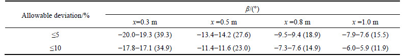
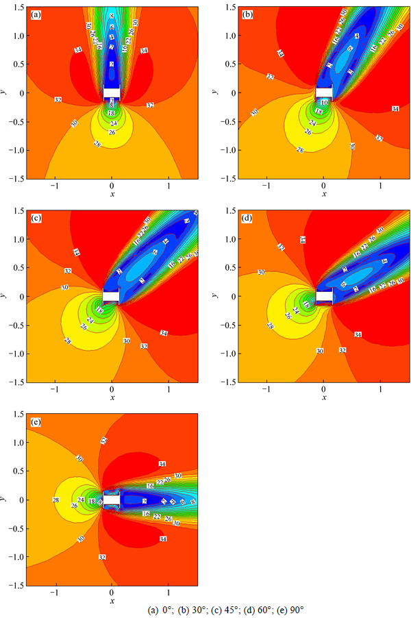
Fig. 9 Velocity contours (unit: m/s):
At the wind direction of 45��, the zone affected is the largest, while the smallest effect zone occurs for wind directions of 0�� and 90��, and the two zones almost have the same dimension. Subsequently, due to the shielding influence of the steel pole, there is a large region with a very low velocity. At the wind direction of 45��, the zone affected is the largest as well. The shorter the distance from the steel pole, the lower the speed in that zone. Except of these deceleration zones, two acceleration regions are accompanied by the sides of the pole. As a result, a beautiful velocity contour, a ��two-sided petal acceleration region�� with a ��central pistil deceleration zone��, comes into being (see Fig. 9).
Figure 10 shows the streamlines around the cross- section. Meanwhile, some vortices exist in the corners of and behind the steel pole. At the wind direction of 0�� and 90��, two clear and symmetrical vortices are presented on the windward side of the pole, as shown in Fig. 9. However, at the wind direction of 45��, there are still two clear vortices coming out. The vortices are much larger and non-symmetrical, with a certain connection between the both.
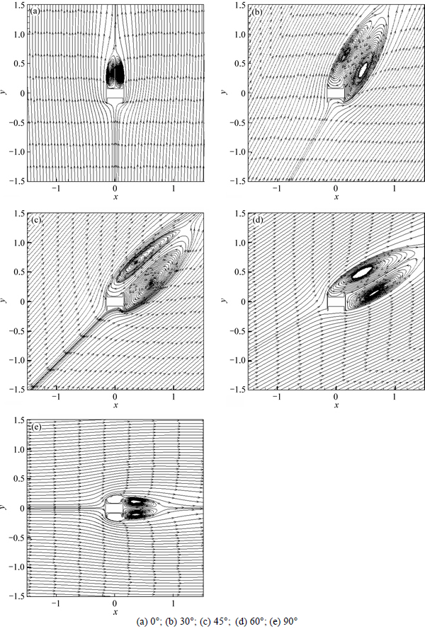
Fig. 10 Streamlines:
After the analysis of flow fields around the pole on the z=0 m plane, the velocity distributions of lines at the distance of 0.5 m, 0.8 m and 1.0 m, respectively, are studied to find a reasonable location between the pole and wind speed sensors. The positions of the lines are depicted in Fig. 11 (a). The distributions of velocity ratio RU are demonstrated in Figs. 11(b)-(c) for the wind direction of 45�� and 90�� respectively, with the location labels of wind speed sensors. The distance between two sensors is 0.8 m, 2.67L. It can be deduced that the velocity ratio RU fluctuates less on the upstream side than on the downstream side. The maximums of RU of lines on the downstream side are larger, especially for the direction of 90��, but their minimums are close to 0. And the shorter the distance from the pole, the greater the impact on the velocity ratio RU. At 45��, the region of influence is bigger and has a non-symmetrical distribution, which is accordance with that shown in Fig. 8. However, at 90��, the curve has a symmetric distribution with respect to the line at y/L = 0.
Thus, based on the positions of sensors in Figs. 11(b)-(c), the results are listed in Table 2. Without considering the case of disturbance between the sensors themselves, for the sensor-1, when d �� 0.8 m along the negative direction of the x axis, the measurement results can��t meet the requirement for all wind directions. As d=-0.5 m with ����45��, and d=-0.8 m with ����30��, RU under each condition is beyond the allowable measured deviation of ��10%. However, as d=-1.0 m, the measurement results can meet all of wind directions.
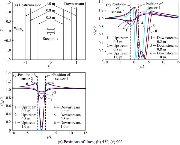
Fig. 11 RU along lines under different distances:
Table 2 RU of lines at different positions

After that, sensors put at the positive direction of the x axis. For the shield effect of the steel pole, the position of sensor-1 isn��t suitable. As to sensor-2, when d=-0.8 m or -1.0 m, the measurement results are well done. While sensor-2 locates at the positive of x axis, due to the effect of accelerated air, RU is more than 1.0 with the maximum of 1.21, where isn��t suitable for installing sensors. Thus, it is suggested that d=1.0 m and the sensors locate on the upstream side.
6 Conclusions
1) It is very necessary to take the flow field around a sensor into consideration to analyze the interaction disturbance of flow field between two wind speed sensors, when one monitoring point has two sensors. In front of the sensor, the speed meets the allowable measured deviations of 10% based on the incoming flow speed. However, behind the sensor, a region with low speed and a peak value of the wind speed comes into being. When the virtual wind speed sensor is closer to it, the influence angle is bigger. However, from the distance of 0.3 m to that of 1.0 m, the most adverse angles are not in excess of ��20�� (40��), and the distance between two wind speed sensors over 0.8 m would be better for the measurement of sensors.
2) The steel poles have a significant influence on the measurement results of wind speed sensor. Installing the wind speed sensor around it, the closer the distance, the more the effect on the measurement. Due to the blockage effect and the shielding influence of the steel pole, a beautiful velocity contour, a ��two-sided petal acceleration region�� with a ��central pistil deceleration zone��, comes into being. Located in upstream side, the distance away from the mast is greater than or equal to 1.0 m, and the velocity ratios of sensor all meet the measurement deviation of 10% under different wind directions. On the contrary, they aren��t all agreeable.
3) From the perspective of ranges of influence under different wind directions, at the wind direction of 45��, the zone affected is the largest, while the smallest effect zone occurs for wind directions of 0�� and 90��, and the two zones almost have the same dimension. Meanwhile, some vortices exist in the corners of and behind the steel pole. At the wind directions of 0�� and 90��, two clear and symmetrical vortices are presented on the windward side of the pole. At the wind direction of 45��, there are still two clear vortices coming out, but the vortices are much larger and non-symmetrical, with a certain connection between the both.
4) Thus, it is proposed that the distance between two wind speed sensors is 0.8 m at least, and the interval between sensors and the steel pole is more than 1.0 m with the sensors located on the upstream side.
References
[1] ANDERSSON E, HAGGSTROM J, SIMA M, STICHEL S. Assessment of train-overturning risk due to strong cross winds [J]. Proceedings of the Institution of Mechanical Engineers, Part F: Journal of Rail and Rapid Transit, 2004, 218(F3): 213-223.
[2] FUJII T, MAEDA T, ISHIDA H, IMAI T, TANEMOTO K, SUZUKI M. Wind-induced accidents of train/vehicles and their measures in japan [J]. Quarterly Report of Railway Technical Research Institute, 1999, 40(1): 50-55.
[3] SUZUKI M, TANEMOTO K, TATSUO M. Aerodynamics characteristics of train/vehicles under cross winds [J]. Journal of Wind Engineering and Industrial Aerodynamics, 2003, 91(1): 209-218.
[4] SANQUER S, BARRE C, VIREL MD, CLEON L M. Effect of cross winds on high-speed trains: Development of a new experimental methodology [J]. Journal of Wind Engineering and Industrial Aerodynamics, 2004, 92: 535-545.
[5] BOCCIOLONE M, CHELI F, CORRADI R, MUGGIASCA S, TOMASINI G. Crosswind action on rail vehicles: Wind tunnel experimental analyses [J]. Journal of Wind Engineering and Industrial Aerodynamics, 2008, 96(5): 584-610.
[6] CHELI F, RIPAMONTI F, ROCCHI D, TOMASINI G. Aerodynamic behaviour investigation of the new EMUV250 train to cross wind [J]. Journal of Wind Engineering and Industrial Aerodynamics, 2010, 98(6/7): 189-201.
[7] CHELI F, CORRADI R, ROCCHI D, TOMASINI G, MAESTRINI E. Wind tunnel tests on train scale models to investigate the effect of infrastructure scenario [J]. Journal of Wind Engineering and Industrial Aerodynamics, 2010, 98(6/7): 353-362.
[8] DIEDRICHS B, SIMA M, ORELLANO A, TENGSTRAND H. Crosswind stability of a high-speed train on a high embankment [J]. Proceedings of the Institution of Mechanical Engineers, Part F: Journal of Rail and Rapid Transit, 2007, 221(2): 205-225.
[9] SCHOBER M, WEISE M, ORELLANO A, DEEG P, WETZEL W. Wind tunnel investigation of an ICE 3 end car on three standard ground scenarios [J]. Journal of Wind Engineering and Industrial Aerodynamics, 2010, 98(6/7): 345-352.
[10] TIAN H Q. Research progress in railway safety under strong wind condition in China [J]. Journal of Central South University: Science and Technology, 2010, 41(6): 2435-2443. (in Chinese)
[11] LIU T H, ZHANG J. Effect of landform on aerodynamic performance of high-speed trains in cutting under cross wind [J]. Journal of Central South University, 2013, 20(3): 830-836.
[12] REZVANI M A, MOHEBBI M. Numerical calculations of aerodynamic performance for ATM train at crosswind conditions [J]. Wind and Structures, 2014, 18(5): 529-548.
[13] TOMASINI G, GIAPPINO S, CORRADI R. Experimental investigation of the effects of embankment scenario on railway vehicle aerodynamic coefficients [J]. Journal of Wind Engineering and Industrial Aerodynamics, 2014, 131: 59-71.
[14] HEMIDA H, KRAJNOVIC S. LES study of the influence of the nose shape and yaw angles on flow structures around trains [J]. Journal of Wind Engineering and Industrial Aerodynamics, 2010, 98: 34-46.
[15] ZHANG J, LIANG X F, LIU T H, LU L F. Optimization Research on aerodynamic shape of passenger car body with strong crosswind [J]. Journal of Central South University: Science and Technology, 2011, 42(11): 3578-3584. (in Chinese)
[16] ZHANG J, GAO G J, LI L J. Height optimization of windbreak wall with holes on high-speed railway bridge [J]. Journal of Traffic and Transportation Engineering, 2013, 13(6): 28-35. (in Chinese)
[17] ZHANG T, XIA H, GUO W W. Analysis on running safety of train on bridge with wind barriers subjected to cross wind [J]. Wind and Structures, 2013, 17(2): 203-225.
[18] AVILA-SANCHEZ S, PINDADO S, LOPEZ-GARCIA O, SANZ- ANDRES A. Wind tunnel analysis of the aerodynamic loads on rolling stock over railway embankments: The effect of shelter windbreaks [J]. The Scientific World Journal, 2014, 2014: 1-17.
[19] GONG J, WANG P. Research on gale monitoring & early warning system of high-speed railway [J]. High Speed Railway Technology, 2012, 3(1): 5-8, 14. (in Chinese)
[20] HOPPMANN U, KOENIG S, TIELKES T, MATSCHKE G. A short term strong wind prediction model for railway application: design and verification [J]. Journal of Wind Engineering and Industrial Aerodynamics, 2002, 90: 1127-1134.
[21] SNCF I/SYSTRA. Consulting report of CHI high-speed railway on engineering design [R]. 2004
[22] JIA Y X, MEI Y G. Development of strong winds early warning system in japan high- speed railway [J]. Railway Locomotive & Car, 2008, 28(4): 16-19. (in Chinese)
[23] YE W J, LIU H G, XUE J. Monitoring, forecasting and early warning system for severe weather along the railway line [J]. Bimonthly of Xinjiang Meteorology, 2001, 24(6): 25-27. (in Chinese)
[24] MIAO X J, ZENG X K, GAO G J. Wind anemometer location choosing near railway embankment [J]. Journal of Central South University: Science and Technology, 2013, 44(10): 4328-4333. (in Chinese)
[25] GAO G J, ZHANG J, XIONG X H. Location of anemometer along Lanzhou-Xinjiang railway [J]. Journal of Central South University, 2014, 21(9): 3698-3704.
[26] BOURIS D, BERGELES G. 2D LES of vortex shedding from a square cylinder [J]. Journal of Wind Engineering and Industrial Aerodynamics, 1999, 80: 31-46.
[27] DURAO D, HEITOR M, PEREIRA J. Measurements of turbulent and periodic flows around a square cross-section cylinder [J]. Experiments in Fluids, 1988, 6: 298-304.
(Edited by YANG Hua)
Foundation item: Projects(U1334205, 51205418) supported by the National Natural Science Foundation of China; Project(2014T002-A) supported by the Science and Technology Research Program of China Railway Corporation; Project(132014) supported by the Fok Ying Tong Education Foundation of China
Received date: 2015-10-13; Accepted date: 2016-03-09
Corresponding author: XIONG Xiao-hui, Lecture, PhD; Tel: +86-13787099389; E-mail: xhxiong@csu.edu.cn
Abstract: In order to consider the influence of steel pole on the measurement of wind speed sensors and determinate the installation position of wind speed sensors, the flow field around wind speed sensors was investigated. Based on the three-dimensional steady Reynolds-averaged Navier-Stokes equations and k-�� double equations turbulent model, the field flow around the wind speed sensor and the steel pole along a high-speed railway was simulated on an unstructured grid. The grid-independent validation was conducted and the accuracy of the present numerical simulation method was validated by experiments and simulations carried out by previous researchers. Results show that the steel pole has a significant influence on the measurement results of wind speed sensors. As the distance between two wind speed sensors is varied from 0.3 to 1.0 m, the impact angles are less than ��20��, it is proposed that the distance between two wind speed sensors is 0.8 m at least, and the interval between wind speed sensors and the steel pole is more than 1.0 m with the sensors located on the upstream side.
