J. Cent. South Univ. (2018) 25: 315-330

DOI: https://doi.org/10.1007/s11771-018-3739-2

A hybrid algorithm based on tabu search and large neighbourhood search for car sequencing problem

ZHANG Xiang-yang(张向阳)^{1, 2, 3}, GAO Liang(高亮)², WEN Long(文龙)², HUANG Zhao-dong(黄兆东)^{1, 3}

1. Faulty of Maritime and Transportation, Ningbo University, Ningbo 315211, China;

2. State Key Laboratory of Digital Manufacturing Equipment & Technology, Huazhong University of Science & Technology, Wuhan 430074, China;

3. National Traffic Management Engineering & Technology Research Centre Ningbo University Sub-center, Ningbo University, Ningbo 315211, China

Central South University Press and Springer-Verlag GmbH Germany, part of Springer Nature 2018

Abstract:

The car sequencing problem (CSP) concerns a production sequence of different types of cars in the mixed-model assembly line. A hybrid algorithm is proposed to find an assembly sequence of CSP with minimum violations. Firstly, the hybrid algorithm is based on the tabu search and large neighborhood search (TLNS), servicing as the framework. Moreover, two components are incorporated into the hybrid algorithm. One is the parallel constructive heuristic (PCH) that is used to construct a set of initial solutions and find some high quality solutions, and the other is the small neighborhood search (SNS) which is designed to improve the new constructed solutions. The computational results show that the proposed hybrid algorithm (PCH+TLNS+SNS) obtains 100 best known values out of 109 public instances, among these 89 instances get their best known values with 100% success rate. By comparing with the well-known related algorithms, computational results demonstrate the effectiveness, efficiency and robustness of the proposed algorithm.

Key words:

car sequencing problem; large neighborhood search; tabu search; ratio constraint；

Cite this article as:

ZHANG Xiang-yang, GAO Liang, WEN Long, HUANG Zhao-dong. A hybrid algorithm based on tabu search and large neighbourhood search for car sequencing problem [J]. Journal of Central South University, 2018, 25(2): 315–330.

1 Introduction

The car sequencing problem (CSP) involves determining an order of cars for each workday’s production in a mixed-model assembly line. A mixed-model assembly line makes various types of cars to be assembled on the same line. Each type of car is combined with several selected options such as sunroof or air conditioner, and common components. The assembly of the options is labor intensive, and the assembly time is usually larger than for common components. Therefore, special work stations are designed for assembling the options. The option ratio constraints stand for the capacities of these work station (e.g., p_o/q_o stands for no more than p_o cars permitted having o options in any subsequence of q_o successive cars). The associated types with the option should not be arranged in successive positions in a sequence so as to avoid overload of the work station. Therefore, the CSP is proposed to tackle this situation.

The CSP is NP-hard in the strong sense [1]. It is described as one of a constraint satisfaction problems at first, and some public instances of the CSP are available to testify the performance of constraint solvers [2]. The constraint satisfaction problem concerns the assignment of values to a set of variables from their respective domains in order to satisfy all the constraints of the associated variables. A sequence acts as a solution and each position of the sequence is deemed as a variable, so the purpose of the CSP is to determine how to assign an appropriate available type to every position without creating any violation. However, when some difficult instances have no feasible solution (that all capacity constraints must be met), the sum of violations is used to evaluate the quality of that solution. Therefore, a decision CSP is changed into an optimization CSP by relaxing the constraints of the options and turning them into the objective function.

Different exact methods from constraint programming (CP) and operation research (OR) have been applied to this well-known problem. Some CP solvers, using a systemic search to find feasible solutions in a tree-like space can also solve such instances that have no feasible solutions. Some specialized filtering algorithms are efficient in dealing with some hard constraints, but the limitation of filtering algorithms is that they cannot solve large scale instances in limited time [3]. FLIEDNER and BOYSEN [4] proposed a specialized Branch & Bound algorithm after they exploited the structure of the CSP. Although the proposed method might not be applicable to real production, it provided structural insights which can be applied to existing heuristics. ARTIGUES et al [5] proposed and compared hybrid CP/SAT models for the CSP against several SAT-encodings. They got most of the best known values in the public instances but some easy instances, such as 200-02 and 400-01, cannot be solved within 20 min. Recently, GOLLE et al [6] developed an iterative beam search (IBS) showing competitive results. The IBS is based on a truncated breadth-first search in an incomplete search space. They claimed their algorithm was also appropriate to the optimization of the CSP. However, ZHANG et al [7] used several simple constraint propagation rules nested in a parallel heuristic framework to get the competitive results. Moreover, SIALA et al [8] systemically classified the heuristic rules in tree search. They showed that some heuristics combining simple filtering rules work better than the proposed solvers in the tree search, so this combination is suggested to be embedded within local search.

Besides such exact methods that systematically search for solutions in tree search space, various heuristics were studied that provide an opportunistic way to search approximate optimal solutions. Among these heuristics, constructive approaches and local search approaches are two main directions to improve solutions. For the former, ant colony optimization (ACO) [3] and a greedy randomized adaptive search procedure (GRASP) [9] iteratively reconstruct the solution from partial solution via acquired knowledge in the previous operation, but their performance is not competitive. For the latter, most of these methods were published after the ROADEAF’2005 challenge which was initiated to solve the expanded CSP [10]. CORDEAU et al [11] proposed an iterated tabu search (ITS) for solving the special CSP, and the algorithm showed a good performance. BRIANT et al [12] presented a greedy approach and simulated annealing (SA) which showed its efficiency in the challenge. However, these proposed algorithms focus mainly not on the constraints of the options, but on multi objectives. Moreover, most of these effective algorithms are the combinations of two or more different algorithms. These hybrid algorithms reached a good performance in mixed-model assembly [13]. PERRON et al [14] testified the portfolio of algorithms. They incorporated several local search solvers within the large neighborhood search (LNS) framework and got some competitive solutions in some public instances. GRAVEL et al [15] put forward an ACO combined with a local search (ACO+LS) that showed a high performance in the public instances. PRANDTSTERTTER and RAIDL [16] proposed a hybrid algorithm that combines an integral linear programming and a variable neighborhood search (ILP+VNS). They claimed the hybrid algorithm outperforms other approaches in the challenge. ZINFLOU et al [17] proposed a genetic algorithm which incorporates a crossover using integral linear programming model (ILP+GA). Moreover, THIRUVADY et al [18] proposed an algorithm consisting of CP, beam search and ACO, and the algorithm better than any of the other combinations. Recently, they tried a hybrid algorithm named Lagrangian-ACO [19] which even outperforms the method of PRANDTSTERTTER and RAIDL [16]. Although different algorithms verified their superiority to others in some characters, the algorithm combinations showed their advantages of solving the CSP, and this deserves further investigation.

Therefore, this work is concerned with the performance of different portfolios of algorithms in order to take full advantages of complementary methods for the CSP. One comes from the combination of tabu search and large neighborhood search (TS+LNS, or TLNS for short). On one hand, TLNS leads to a high performance in the exploring and exploiting of TS, its adaptive neighborhood modification with the help of memory-based strategies. Based on these strategies, one candidate list and two tabu lists assist the selection of a solution to be improved. Then on the other hand, TLNS works as a framework to iteratively improve the current solution by alternately destroying and repairing moves in a very large neighborhood. Moreover, both a parallel constructive heuristic (PCH) in the construction of the solution, and small neighborhood search (SNS), contribute to the improvement of the solution under the TLNS.

The rest of this paper is organized as follows. Section 2 describes the CSP model. The proposed algorithm is described in Section 3, along with some details of techniques used for its implementation. In Section 4, different algorithm combinations are evaluated according to the computation results and a comparison is completed with well-known algorithms. Section 5 concludes the work.

2 Car sequencing problem

This section presents a formal definition of the CSP. Given the above instance, the decision CSP introducessome binary decision variables whose value is 1 if type c is arranged for position t or 0 else. The solution is to evaluate a sequence of variables that satisfying all related constraints. The mathematical model is built with reference to DREXL and KIMMS [20].

                   (1)

                        (2)

  (3)

              (4)

Equation (1) indicates that every position of the solution sequence must arrange exactly only one type. Equation (2) shows that each type must obey its output requirement. Inequalities (3) require

every subsequence of each option must satisfy its ratio constraint, and there are total subsequences.

However, an optimization CSP is commonly accepted when a violation is inevitable. In this condition, the option constraints are relaxed and become soft constraints. Therefore, the purpose of the CSP is to obtain a solution sequence leading to the least violations. Usually a “sliding windows” technique is applied to counting the number of violated subsequences but some flaws used in the objective function have been pointed out [4]. To compare with other methods, we continue to use this technique into the objective function. An objective function is put forward to evaluate the quality of the solution. The commonly accepted objective function, shown in Eq. (5), computes the number of subsequences that violate the related ratio constraints.

(5)

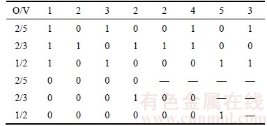
A simple example is given in Table 1. A sequence of 8 cars is shown in top row, with a number in each slot of the sequence denoting a type of car. There are 5 types and each is a combination of 3 options. A type is expressed with a column vector of 3 dimensions. For example, [0 0 1]^T denotes type 5 which has option 3. So, a sequence consisting of types can also be expressed with a matrix of 0-1 shown in rows 2–4, in which the number of rows is the number of options and the number of columns is the total number of cars. Each number in the last three rows denotes whether the corresponding subsequence of one option violates its ratio constraint or not. There are 17 subsequences for 3 options. Here, 2 violations occur. One subsequence (2, 2, 4) violates ratio 2/3 and the other subsequence (5, 3) violates ratio 1/2. If we exchange types 4 and 5 in the sequence, however, the new sequence has no violations.

Table 1 Violations using traditional and improved objective functions for a sequence

3 A hybrid algorithm

This section prescribes a hybrid algorithm PCH+TLNS+SNS for the CSP. TLNS, as the framework of the hybrid algorithm, is proposed after the introduction of LNS. Next, the destroying and repairing methods of TLNS are introduced, both of which are used to construct the large neighborhood and complete the search respectively. In addition, PCH and SNS are sequentially presented, both of which are integrated into TLNS.

3.1 Large neighborhood search

The basic idea of LNS proposed by SHAW [21] is that an initial solution is gradually improved by alternately destroying and repairing the current solution in a very large neighborhood. In other words, LNS iteratively improves the solution by relaxing parts of variables and reassigning values to them. PISINGER and ROPKE [22] presented the framework of LNS shown in Algorithm 1.

In Algorithm1, an initial solution χ is given as an input in line 1, treated as the best solution χ^b in line 2. A loop from line 3 to line 7 is the main iteration process. In line 4, the current solution χ is destroyed using the function d(·) and then is repaired using the function r(·), so the temporary solution χ^t is acquired from the neighborhood r(d(·)). In line 5, the temporary solution χ^t is compared with the current solution χ to determine if the former can be accepted under the accept function and will replace the latter if affirmed. Line 6 checks if χ^t is better than χ^b according to the objective function c(χ); if so it updates the best solution. The iteration process stops when the termination condition is met in line 7 and the best solution is returned in line 8.

3.2 A hybrid algorithm PCH+TLNS+SNS

As the framework of the hybrid algorithm, TLNS exploits the characters of LNS and TS. A general variation of LNS is achieved by using a fast restart strategy and accepting the equivalent intermediate solutions [23]. LNS is very flexible and can be easily integrated into any local search heuristic like SA or TS [24] or exact methods such as standard backtracking procedure [23]. As emphasized by PISINGER and ROPKE [22], more freedom is allowed in the repair phase, an existing construction heuristic can be quickly turned into a repair heuristic and a destroy method based on random selection is easy to complete [22]. Hybrid algorithms based on LNS rather than simple LNS tended to evolve, and these hybrid algorithms are appropriate to solve the difficult combination optimization problems [25]. TS is a general heuristic that guides a search to obtain good solutions for difficult combination problems. In addition, tabu lists serve as a diversify avenue to solve the CSP given by Cordeauet et al [11], GAVRANOVI [26] and ZUFFEREY [27], candidate lists also provide a memory-based strategy to modify the adaptive neighborhood on which TS relies to intensify the searching [28]. TS is incorporated into LNS to form TLNS in order to escape searching the redundant solutions and to navigate the searching toward the more promising space. In TLNS, the tabu list is used to prohibit investigation of the redundant solutions, while the candidate list confines the current solution to a list of high quality solutions.

As mentioned above, a fast constructive heuristic (CH) not only iteratively reconstructs a solution in the repair function, but also acts as an initial solution in the TLNS. However, to improve the quality of initial solutions and to accelerate the iteration process, PCH replaces CH for the input to TLNS. Moreover, SNS has the capacity of quickly finding local optima solutions, so it supplements the capacity of intensive searching in the repair stage of TLNS. Therefore, the hybrid algorithm PCH+ TLNS+SNS consisting of TLNS, PCH and SNS is proposed to exploit the performance of the portfolio of algorithms. The framework of the hybrid algorithm is presented in Algorithm 2.

In Algorithm 2, a candidate list CandiSet is a set of initial solutions acquired with a PCH, and two tabu lists, SolSet and PartSet, are set empty separately in line 1. In line 2, the solution with the least violations in CandiSet is selected and acts as the best solution χ^b. An outer loop from line 3 to line 13 repeats the iteration process. In line 4, an alternative solution χ is selected from CandiSet, an elite set which continuously absorbs the high quality solutions during the search; χ is subsequently abandoned to the tabu solution list SolSet to escape repeating operation later. The nested inner loop from line 5 to line 12 is responsible for most tasks of the TLNS. In line 6, a partial solution χ^p is obtained by destroying χ and put into another tabu list PartSet that collects a number of partial solutions to avoid repeating repair in later searches. As for the CSP, we randomly extract a partial solution from the whole solution. The partial solution remains unchanged in the construction of a new solution χ^r in line 7. A heuristic uses some filtering rules to quickly construct a new solution which will be introduced in next section. If the solution χ^r is accepted according to an accept function, it will be added into CandiSet; otherwise it will go back to step 5 and the inner loop will restart instantly in line 8. The best solution χ^b will be updated by χ^r if it is better than χ^b in line 9. Besides the construction in the repair, SNS(χ^r) improves χ^r and obtains some new solutions like χ^e in line 10; concurrently, CandiSet will be updated if χ^e is no worse than χ^r during the search. The best solution χ^b will be replaced with χ^r when the latter is much better in line 11. The inner loop stops after all iterations have completed or no better solution occurs in line 12, and the outer loop terminates according to the stop criteria in line 13. Line 14 outputs the best solution χ^b.

3.3 Neighborhood construction and search

The critical issue of applying TLNS to the CSP is how to construct appropriate neighborhoods and how to accomplish the search efficiently. Two points must be emphasized to achieve these two goals. Firstly, destroy and repair methods used in the CSP should embody the characteristics of ratio constraints. Secondly, the design of destroy and repair methods should consider their overall effectiveness, in other words, the two methods should be put together in the program.

Usually, the assignment to a variable in the sequence should meet the ratio constraints of all options in several contiguous subsequences. Also, this assignment should conform to the types’ output requirement. Hence, when facing tight constraints, the type arrangement to a certain variable is difficult to change into the assignment of another type without violations increasing. Using CH as a repair function, it is possible to reassign to several contiguous variables instead of only one isolated variable in the current solution.

3.3.1 A destroy method

To avoid obtaining the same solution in the reconstruction, the destroy method is used to select randomly the middle part of the solution as the fixed part whose values are kept unchanged. There are two reasons for this: Firstly, different partial solutions can result in different assignments to the remaining variables as each assignment must obey the accomplished arrangement of variables. Secondly, this selection is beneficial to the reconstruction. When the variables at the head and tail parts are selected to reassign, the easier types at the head can counteract the harder ones at the tail in the reconstruction.

A destroy method presented here exploits the neighborhood through a systematic strategy. The strategy enlarges the neighborhood increasingly by recurrently changing the two terminals’ positions of the partial solution. When a part of the current solution is selected randomly as the destroyed partial solution and then it is put in the tabu partial solution list, the number of the selections is so large that a huge number of iterations should be prohibited. To ensure diversity of the search, a systematic strategy that obeys a specific order is designed in addition to applying the tabu list strategy.

A systematic strategy of partial solution construction is described. A parameter k expresses the number of the sampling positions in the solution χ, and the sampling positions satisfy 1≤π₁<π₂<…<

π_k≤n. Then, a partial solution is expressed with for 1≤ithat has the minimum neighborhood. Next, with k replaced by k–1 and selected, the neighborhood is enlarged accordingly. Thirdly, by changing the first position, is selected and this variation with i and j continues until the criterion is met aswhere D is the minimum length of the partial solution. Lastly, this transformation keeps going until a better solution is achieved or all neighborhoods are searched. As mentioned above, all partial solutions obtained should be ranked in the tabu list, PartSet, so each of them should compare with the existing partial solutions in the list to avoid repeating operations.

3.3.2 A repair method

CH is used as the repair method of TLNS, it reconstructs the solution from a partial solution, and the reconstruction also acts as an improvement of the solution. The operation of CH resembles PCH, but the latter constructs a set of initial solutions in one operation and these initial solutions are constructed from void. Although there is a small difference between the partial solution construction and the initial solution construction, one point deserves attention. This is that if the violations of a partial solution are greater than that of the upper boundary of the candidate list, the construction will terminate. A general principle of CH is expressed in Algorithm 3 and more details about the construction will be given in next section.

Algorithm 3 ignores the selection process and mainly focuses on the basic framework of the algorithm. Line one shows four input parameters objBest, carNum, parti and ParSet, these are the best objective value, number of cars, the partial solution and the tabu partial solution set. The procedure starts with a check whether parti will be rejected or not. If it belongs to PartSet, the procedure returns an empty solution f in line 2. Otherwise, the tabu list PartSet is updated by adding parti in line 4. The loop of lines 5 to 8 gives the main body of the construction. In line 6, a position variable is assigned a type in each step to get a new partial solution, parti. In line 7, another judgment is done as to whether the objective value of parti is larger than worst(candiSet), the worst objective value of the list; if so the procedure returns an empty solution. In the end, a whole solution χ is returned in line 10.

3.4 Parallel constructive heuristic (PCH)

CH can not only reconstruct a solution from a partial solution derived from the destroy function, but also construct initial solutions from void. However, the neighborhood of LNS is too large to be searched explicitly. In order to construct high quality solutions quickly and enhance the robustness of the algorithm, PCH is proposed to construct a set of initial solutions as the input of TLNS rather than generating randomly an initial solution using CH.

As the input of TLNS, a set of solutions are constructed using a PCH, and the set of solutions can be set as the candidate list. The parallel scheme aims to get a best solution quickly by comparing these solutions after the construction. The same heuristic and principle is used to construct every solution except for the first variable’s assignment with different type. Each solution is constructed using a heuristic that incorporates three filtering rules and three greedy functions into the process of the construction. To narrow the variable domain, these filtering rules rule out some unpromising solutions in advance based on constraint propagation [6, 8]. Moreover, three greedy functions are used to further narrow the variable domain and help the complement of the assignment with the greedily style [7]. Figure 1 shows the general flow chart of PCH to construct initial solutions for the CSP.

In Figure 1, in order to achieve a high quality solution quickly, three filtering rules cooperate with three greedy functions, and they sequentially operate until the current variable is assigned a type of car. The first filtering rule expels the types used up in the partial solution, so the domains of the remaining position variables are updated with the remaining types of the cars. After the filtering rule used, the first greedy function selects the types with the minimum violations of the current subsequences, computed as Eq. (6), so the domain is updated again. Next, the second filtering rule and the third one update consecutively the domain. The second rule expels the types for whose assignment to the current position variable can definitely lead to the violations of the remaining cars. The third rule is used to avoid continuous violations of the adjacent variables, so it should rule out the types that could result in the next position variable’s violation. The second greedy function selects the types holding the biggest value of DSU [3] (dynamic sum of options utilization rates, which expresses the difficulty of the type to be assigned after the partial solution), and it updates the domain in order to arrange the most difficult type firstly. The third function aims to complete the assignment by selecting the type with the biggest change of the difficulty between the partial solution and the remaining cars.

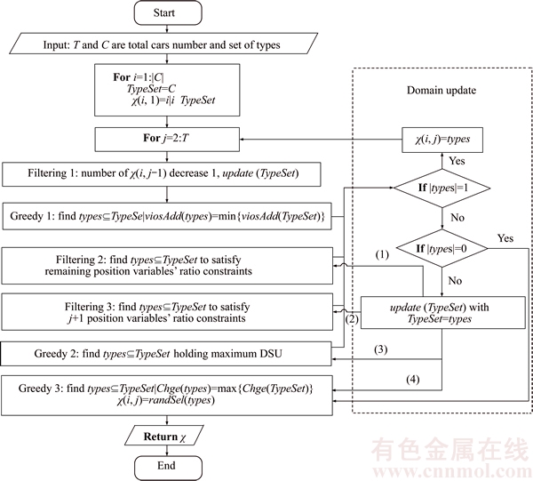
Figure 1 Parallel construction heuristic to construct initial solutions for CSP

   (6)

Moreover, three circumstances should be dealt with after using the last two filtering rules or the first two greedy functions shown in the right dashed line box of Figure 1, which expresses the process of the domain update. The first one is that only one type left, so the type will be assigned to the current variable. The second one expresses no type left, then the domain keeps unchanging, and third greedy function helps the complement of the assignment. The third one is applied when more than one type is left, the domain should be updated further with the next filtering rule or next greedy function. Note that, one arrow that marked with (1), (2), (3) or (4) toward to one of the last two filtering rules or the last two greedy functions, denotes the output of the last filtering rule or function.

3.5 Small neighborhood search (SNS)

As proposed by PERRON et al [14], local search moves as swap, insert and invert are easily integrated in the TLNS architecture. Therefore, SNS is incorporated into the hybrid algorithm to improve the reconstructed solution. SNS is very useful to improve the current solution because of its efficiency, so three basic operators, which are swap, insert and invert, are used after the construction. Figure 2 is a sketch map that explains above.

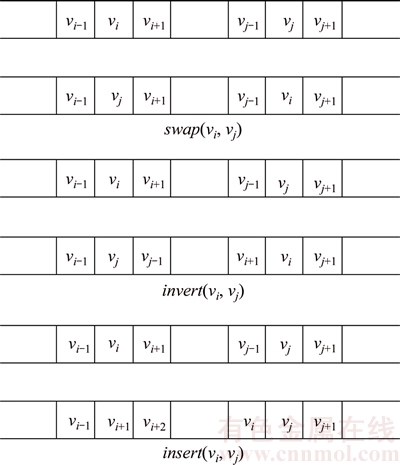
Figure 2 Small neighborhood search for CSP

SNS follows the construction and the operators iteratively improve the current solution by pivoting on the positions which result in violations. Therefore, some equal, or better, solutions are put into the candidate list, to diversify the search. To avoid redundant operations, the violated position acts as a central axis pivoted by other positions. Once a better solution is acquired, the candidate list is updated, and then another improvement begins. More details are given in Algorithm 4.

In line 1, two input parameters, χ and CandiSet, are the current solution and the candidate list respectively. Lines between 2 to 14 describe the process of iteration, during which new improved solutions occur. Firstly, the set of all violation positions π₁, is separated from set of all positions π in line 3. Next, if a violated position t can be extracted from π₁, in line 4, then π₁ and π are updated by taking out t in line 5. From line 6 to line 13, for the violated position t and each position k, three operators are implemented in order. For example, if , which means an equivalent or a better solution is acquired, the new solution χ^t will be put into a candidate list in line 7, and it will replace the current solution and restart the iteration with the new one if it improves the current solution in line 8. On completion of all iterations, solution χ is returned.

4 Computational experiments

4.1 Experimental setup

In order to test the validity of the algorithm, the CSPLib (www.csplib.org) benchmark library has been constructed [2]. This is an online library of constraint satisfactory problem. 109 problem instances are divided into three sets based on utilization rates and instance scale. Set 1 consists of 70 instances of different levels of difficulty by the optional utilization rates. Every instance consists of 200 cars, 5 options that are combined to form 17 to 30 types, solved without violation. Set 2 consists of 9 instances with 100 cars, 5 options and 19-26 types. Among them, only four instances have zero violations [26]. In fact, this set is somewhat difficult to solve because some option utilization rates exceed 0.95, or even equal to 1. Set 3 is composed of 30 larger instances with 200–400 cars, 5 options and 19–26 types. Set 3 is more difficult to solve than Set 2, and 7 instances have zero violation solutions. The proposed algorithm is implemented in MATLAB 12.0 and tested on Core^TM i3 CPU 2.13 GHz and 2.0 GB RAM.

4.2 Results and performance of algorithm portfolio

Above all, in order to show the effects of the combinations of algorithms, the different algorithm models are firstly distinguished. For example, whether PCH/CH is beneficial to the performance, and whether SNS can improve the quality of solution, and how their coalition influences the performance of TLNS. TLNS works as the main body of PCH+TLNS+SNS. With TLNS, a randomly generated solution is used as the input of TLNS，and no SNS and no PCH is used in the repair stage.

4.2.1 Set 1

For Set 1, TLNS is of no use because all 70 instances can get zero violation solutions every time in less than 0.2 s using only CH for the initial solution. Actually, this set is easy for its low option ratio usage composition and few cars to be sequenced. In addition, no parameter is needed. It shows that CH is effective in dealing with these easy instances without any iteration by putting any type in the first position. Moreover, it is difficult to compare the performance in that the operation is completed in a very short time.

4.2.2 Set 2

Table 2 shows the comparison of 6 different algorithms in the average value, the average time (seconds) and success rate for Set 2. Note that, for an instance, one operation terminates once the best known value is acquired and a time cost is obtained. Columns 1 and 2 show separately the names of 9 instances and their best known values. The next six columns are the different algorithms that are separated into two groups. As shown in Columns 3 and 4, CH+SNS and PCH+SNS belong to the first group in which SNS is used to improve the current solution. CH or PCH are used to construct an initial solution or to construct several initial solutions. The next four columns belong to the second group which uses TLNS as the framework of SNS, PCH and PCH+SNS respectively. Each instance was operated 20 times within 60 s. Four parameters used in the TLNS are the size of candidate list (ss=50), tabu solution list (st=200), tabu partial solution list (sr=2000) and the number of breakpoints (n=cars/10, which means average space between two points is ten positions). The average value, the average time (in parentheses) and success rate that associated with each instance and each algorithm, are shown in the corresponding cell.

Table 2 Average values and average time (s) and success rates of different methods for Set 2 (each instance operated 20 times within 60 s per time)

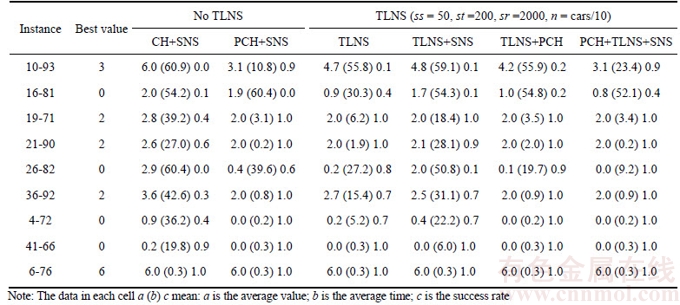
The performance of six algorithms was first compared. In Table 2, the other five algorithms cannot compete with PCH+TLNS+SNS both in the average values and time. The average values of the later is less than or equal to that of other methods. Seven instances in particular, got the best known values except for 10-93 and 16-81, which are more difficult to solve. For 10-93, PCH+SNS can compete with PCH+TLNS+SNS because their average values are equal. In the average time, eight instances except for 16-81, spent less time than the other methods. For 16-81, TLNS spent less time than PCH+TLNS+SNS but its average value is slightly bigger than the former. For the success rates, Table 2 also shows that PCH+TLNS+SNS has higher rates on 9 instances overall compared to that of the other algorithms. For each instance, the success rate is higher than or equal to that of any other algorithms. Note that 7 instances out of 9 got the best known values each time. For 10-93 and 16-81, two difficult instances mentioned in literature, the success rates are still better than that of others. However, these two instances have some contrary characteristics. Although one algorithm got better solutions than the others on one instance, it cannot get better solutions than others in all instances. PCH+TLNS+SNS, however, reaches a compromise such that the success rates of the two instances are kept at a high level.

Another comparison is the effectiveness of each part of the different algorithms, i.e. PCH, TLNS and SNS. Firstly, the algorithms with a PCH are better than those without a PCH, shown in Table 2. See Columns 3 and 4 for CH+SNS and PCH+SNS. See Columns 5 and 7 for TLNS with PCH+TLNS, and Columns 6 and 8 for TLNS+SNS with PCH+TLNS+SNS. Nearly all instances other than 16-81 are superior to their equivalents without PCH in their average values and average time. However, for instance 16-81, it is difficult to compare one algorithm using PCH with the other without a PCH. This is because neither one has an overwhelming superiority over the other. Moreover, for the easier instances such as 21-90, 36-92, 4-72, 41-66 and 6-76, less time was spent using the algorithms with PCH than those without a PCH. In addition, in order to compare the average values and time, the success rates also reflect that the algorithm with PCH has a better performance than the one without it. Secondly, TLNS outperforms the algorithms without TLNS, not only in the average values and time, but also in the success rates. As shown in Table 2, the results of Column 3 and 4 are inferior to Column 6 and 8 respectively. Thirdly, however, the performance of SNS in the algorithms depends on different conditions. By the comparison, PCH+TLNS+SNS outperform PCH+TLNS, but PCH+TLNS+SNS underperforms CH+TLNS. Using PCH, more time was saved because the algorithm can quickly approach the best known values, so SNS could fully utilize the intensity search. At the same time, the advantage of the diversity search can be exerted by TLNS in ample time. Without PCH, more time was wasted on searching the local optimal in the set of low quality solutions.

The parameters of the TLNS were adjusted to the best performance on Set 2. First, the parameter ss was set for 50. We compared four group sizes, 20, 50, 100 and 200. We found that 50 was the most appropriate for the test but others had no significant influence on the results. Also, the parameter st was set for 200 for the same reason. And the parameter sr was set with 2000, which was estimated by the number of breakpoints and the length of the partial solution. The number of breakpoints was set with 5, 10 and 20. The latter two groups had no clear difference, but that with 5. We found that when the number of the breakpoints was set too low, all solutions in the candidate list resulted in failure and the procedure often terminated on some harder instances. In addition, we limited the length of the partial solution to more than half of the solution. This was to save time in the solution construction.

In addition to the parameters, two points need to be noted. One is the acceptance criterion and the other is the method of selection for the candidate solution. For the former, we compared two ways. One allowed the rigorous better solutions than the current solution to enter into the candidate list while the other relaxed the range of the candidate solution by allowing the none-worst solutions to enter into the list. The results indicated that the second way performed the best. For the latter, the method of the selection influences the improvement process. The selection of the high quality solutions can quickly improve the quality of the candidate solutions at the initial stage because more high quality solutions will be created. However, this selection could lose some diversity of the candidate list. Therefore, we used half of the best solutions in the list and the results testified to its good performance.

4.2.3 Set 3

To testify Set 3, the hybrid algorithm PCH+ TLNS+SNS was used to complete the experiment because this algorithm had shown the best performance. Table 3 shows the results of this experiment, in which each instance was tried 20 times within 600 s. For this experiment, we tried different combinations of parameters in the same way as for Set 2 and found the best combination, in which ss was set for 100 and other parameters unchanged. Set 3 has 30 instances. In Table 3, the number of the cars and serial number are shown in Column 1, 6 and 11, and three groups of instances have 200, 300 and 400 cars separately. The best known values are shown in Column 2, 7 and 12, in which 7 instances have zero violation solutions. The next three sets of columns from 3-5, 8-10 and 13-15 are the average value, average time and success rate.

Table 3 Average values, average time (s) and success rates of PCH+TLNS+SNS for Set 3

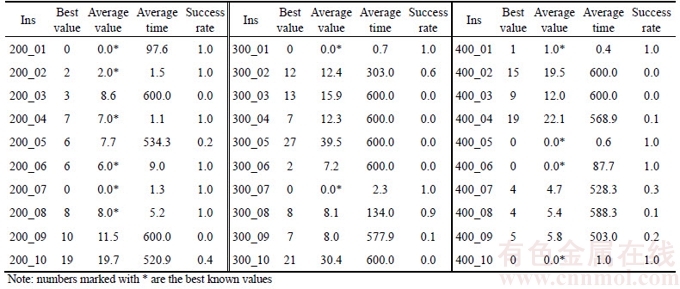
The algorithm PCH+TLNS+SNS got the best known values of 70% instances in relatively short time in Table 3. Among 30 instances, 21 instances got the best known values. The success rates of 12 instances out of 21, whose values are marked *, are 100%. For 7 instances having feasible solutions, the algorithm obtained all their best known values. Note that, the average time expended on 12 instances is no more than 100 s. Actually, 10 of them got their best known values within 10 s, except for 200-01 and 400-06, and 8 instances (200-02/04/07, 300-01/07, 400-01/05/10) only expended about 1 s. PCH accelerated the process, in which the instances got the best known values without any improvement.

In addition to having the high success rates and low time cost, the algorithm also show its high quality of solution. Among the above 21 instances, 9 instances can approach their best known values with a certain probability, and their average values are close to the best known values. Actually, only 6 instances (200-03, 300-04/05/06/10 and 400-02) in Set 3 cannot narrow their gaps. Hence, 6 instances are difficult to solve with PCH+TLNS+SNS.

The time spent on the obtaining of the best known values has no direct relationship with the size of the instances. To show this, two different situations were classified. The first situation shows that only about 2 s were spent on the above 8 instances (200-02/04/07, 300-01/07 and 400-01/05/ 10), and they got the best values in the initial solutions. The other situation shows similar time spent on different instances such as 200-05 and 400-09. The former group got the best known values each time but the latter got the best known values with the same possibility.

4.3 Comparison of experiments

About the efficiency of PCH+TLNS+SNS, we compared it with the well-known algorithms, the references quoted in most of the literature. The comparison mostly focuses on the quality of solutions and the time according to the existing data about Set 2 and 3. Table 4 and Table 5 show the experimental results of PCH+TLNS+SNS completed and contrastive methods, each of which follows a citation that gives the source of quotation and the mostly quoted results.

4.3.1 Set 2

In Table 4, the column on the left shows the methods used, the last row is ours. All other methods in the first column are followed by a citation. Methods marked * generated an initial solution randomly. The top rows show the instance number and best known objective values for Set 2. The remaining cells show the average value and time (seconds) quoted or acquired by the experiments.

Table 4 Comparison of PCH+TLNS+SNS with other methods for Set 2

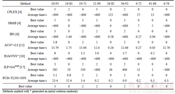
The results of the experiment show 8 instances out of 9 got their best known values. Only one instance, 16-81, obtained an average value that is very close to the best. Actually, only 2 times out of 20 did instance 16-81 get the value of 1 violation. However, for instance 10-93, the most difficult one, PCH+TLNS+SNS got the best known value each time.

Our hybrid algorithm is superior to three exact methods shown in 2-4 rows of Table 4. CPLEX 9.0 is a linear optimization solver, as a benchmark used by SB&B to compare their performance. SB&B, shown in row 3, a special B&B method which treats a partial solution space and defeated the CPLEX in the comparison. The third method IBS, an exact iterative beam search algorithm recently proposed, found a new lower boundary used in the objective function and is superior to SB&B. Our method outperforms IBS on other 7 instances except for instance 16-81 and 26-82. For 26-82, our method spent a little more time although we got the best known value each time. For 16-81, our method cannot compete with IBS in both time taken and value obtained. It is clear to see, however, that these methods spent more than 10 min for 5 instances having no feasible solutions. So, exact methods cannot easily deal with unfeasible instances.

Our hybrid algorithm outperforms the other three hybrid heuristics that are based on iterative improvement on Set 2. The first hybrid method, ACO*+LS, ACO combined into LS framework, which is superior to pure ACO* because it adds a subsequence reversion to improve the current solution. For 5 instances, our method is superior to ACO*+LS either in the average value or time, especially for the more difficult instance 10-93. However, for instances 16-81, 26-82 and 41-66, we cannot compete with the ACO*+LS method. This is because the first instance resulted in a greater average value and the latter two instances required more time to get the best known values. In addition, for instance 4-72, two methods have no clear difference. As for HybrVNS*, an ILP embedded into a general VNS, 5 instances cannot get the best known values every time. Based on GA, the last hybrid heuristic ILP+GA^ncpx incorporates a special crossover operator using ILP. Although ILP+GA^ncpx got their best known values on 9 instances, it required more time than our method with the exception of instance 16-81.

4.3.2 Set 3

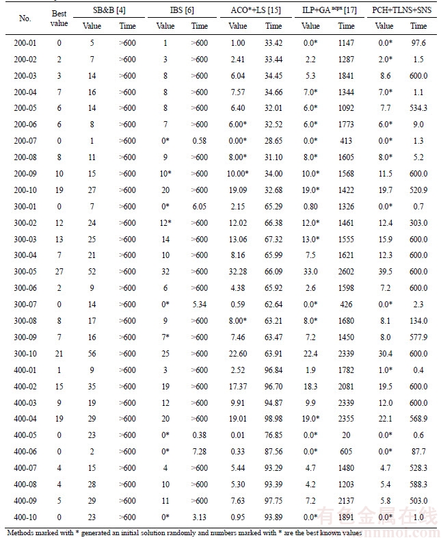
In Table 5, the first two columns list the names and the best-known values. For each method, column 3 to 12 show the average value and time (s). The best values are highlighted by an asterisk *. The last two columns show our results. Two exact methods and two hybrid heuristics were compared with PCH+TLNS+SNS.

As for the first exact method, SB&B cannot compete with ours, not only in the average values obtained, but also in the time spent. Actually, none of thirty instances got the best known value within 10 min. For the second method, IBS is inferior to ours for two reasons. One is that our method got 12 best known values but IBS got only 9 best known. The other reason is that our method used less time than IBS, with which 24 instances used more than 10 min to get the best solutions.

As for the two hybrid heuristics, ACO*+LS can compete well with ours. It outperforms ours in the number of the average values and the average time, but our method outperforms it in the number of best known and the average time required. ACO*+LS has 16 instances with respect to our 14, obtaining the lower average values in less time. Our method got 12 best known values each operation in less time expended, with respect to 5 for ACO*+LS. The last method, ILP+GA^ncpx, spent significantly more time than our method although it got 4 more best known values than ours. For 12 instances, ILP+GA^ncpx spent remarkably more time than our method. In addition, for 400-07/09, our method outperforms ILP+GA^ncpx, since our method used less time for both and got the less average value for 400-09. For the other 16 instances, it is hard to assess whether ILP+GA^ncpx is superior to our method because there is no huge gap but it did expend considerably more time in deriving the average values.

5 Conclusions

We put forward a hybrid algorithm PCH+ TLNS+SNS based on TS and LNS, which is appropriate to solve hard combinational optimization problems having ratio constraints. The hybrid algorithm takes full advantages of TLNS, PCH and SNS in the exploring and exploiting of solutions and the performance of the algorithm is tested and analyzed.

Table 5 Comparison of PCH+TLNS+SNS with other methods for Set 3

The results show the hybrid algorithm gets the best known solutions on public instances with high efficiency and is robust. With total 109 instances of Set 1, 2 and 3, 100 instances got the best known values. Actually, for 39 hard instances of Set 2 and 3, 11 instances got the values with certain probabilities, while 19 instances with 100% success rate within 100 s. As for time cost, 9 out of above 19 instances got the best known values within 1 s, with respect to 17 out of 19 within 10 s. In addition, 9 instances did not get their best known values within 10 min. However, for the 20 instances without 100% success rates, only 6 instances (200-03, 300-04/05/06/10 and 400-02) got the average values, 3 violations more than the best known values.

The proposed hybrid algorithm shows its superiority in the average value and time. For more than two thirds of instances, our algorithm, compared to other methods, can use less time to obtain, or approach, the best known values.

In the future, because our hybrid algorithm shows poor performance on several instances mentioned, the use of different local search operators in the repair function should be further investigated to perfect our algorithm. Moreover, the multi- objective car sequencing problem should be completed with the new hybrid algorithm.

References

[1] KIS T. On the complexity of the car sequencing problem [J]. Operations Research Letters, 2004, 32(4): 331–335.

[2] GENT I P, WALSH T. CSPLib: a benchmark library for constraints [C]// Proceedings of the Principles and Practice of Constraint Programming. Berlin, Germany: Springer Berlin Heidelberg, 1999: 480–481.

[3] GOTTLIEB J, PUCHTA M, SOLNON C. A study of greedy, local search, and ant colony optimization approaches for car sequencing problems [C]// Applications of Evolutionary Computing. Berlin, Germany: Springer Berlin Heidelberg, 2003: 246–257.

[4] FLIEDNER M, BOYSEN N. Solving the car sequencing problem via Branch & Bound [J]. European Journal of Operational Research, 2008, 191(3): 1023–1042.

[5] ARTIGUES C, HEBRARD E, MAYER-EICHBERGER V, et al. SAT and hybrid models of the car sequencing problem [C]// AI and OR Techniques in Constraint Programming for Combinatorial Optimization Problems. Cham, Switzerland: Springer International Publishing, 2014: 268–283.

[6] GOLLE U, ROTHLAUF F, BOYSEN N. Iterative beam search for car sequencing [J]. Annals of Operations Research, 2015, 226(1): 239–254.

[7] ZHANG Xiang-yang, GAO Liang, WEN Long, HUANG Zhao-dong. Parallel construction heuristic combined with constraint propagation for the car sequencing problem [J]. Chinese Journal of Mechanical Engineering, 2017, 30(2): 373–384.

[8] SIALA M, HEBRARD E, HUGUET M J. A study of constraint programming heuristics for the car-sequencing problem [J]. Engineering Applications of Artificial Intelligence, 2015, 38: 34–44.

[9] BAUTISTA J, PEREIRA J, ADENSO-DAZ B. A GRASP approach for the extended car sequencing problem [J]. Journal of Scheduling, 2007, 11(1): 3–16.

[10] SOLNON C, CUNG V D, NGUYEN A, et al. The car sequencing problem: Overview of state-of-the-art methods and industrial case-study of the ROADEF’2005 challenge problem [J]. European Journal of Operational Research, 2008, 191(3): 912–927.

[11] CORDEAU J F, LAPORTE G, PASIN F. Iterated tabu search for the car sequencing problem [J]. European Journal of Operational Research, 2008, 191(3): 945–956.

[12] BRIANT O, NADDEF D, MOUNI G. Greedy approach and multi-criteria simulated annealing for the car sequencing problem [J]. European Journal of Operational Research, 2008, 191(3): 993–1003.

[13] GAO Gui-bin, ZHANG Guo-jun, HUANG Gang, et al. Solving material distribution routing problem in mixed manufacturing systems with a hybrid multi-objective evolutionary algorithm [J]. Journal of Central South University, 2012, 19(2): 433–442.

[14] PERRON L, SHAW P, FURNON V. Propagation guided large neighborhood search [C]// Principles and Practice of Constraint Programming. Berlin, Germany: Springer Berlin Heidelberg, 2004: 468–481.

[15] GRAVEL M, GAGN C, PRICE W. Review and comparison of three methods for the solution of the car sequencing problem [J]. Journal of the Operational Research Society, 2005, 56(11): 1287–1295.

[16] PRANDTSTETTER M, RAIDL G R. An integer linear programming approach and a hybrid variable neighborhood search for the car sequencing problem [J]. European Journal of Operational Research, 2008, 191(3): 1004–1022.

[17] ZINFLOU A, GAGN C, GRAVEL M. Genetic algorithm with hybrid integer linear programming crossover operators for the car-sequencing problem [J]. INFOR: Information Systems and Operational Research, 2010, 48(1): 23–37.

[18] THIRUVADY D R, MEYER B, ERNST A. Car sequencing with constraint-based ACO [C]// Proceedings of the 13th Annual Conference on Genetic and Evolutionary Computation, ACM. 2011: 163–170.

[19] THIRUVADY D, ERNST A, WALLACE M. A Lagrangian- ACO matheuristic for car sequencing [J]. EURO Journal on Computational Optimization, 2014, 2(4): 279–296.

[20] DREXL A, KIMMS A. Sequencing JIT mixed-model assembly lines under station-load and part-usage constraints [J]. Management Science, 2001, 47(3): 480–491.

[21] SHAW P. Using constraint programming and local search methods to solve vehicle routing problems [C]// Principles and Practice of Constraint Programming. Berlin, Germany: Springer Berlin Heidelberg, 1998: 417–431.

[22] PISINGER D, ROPKE S. Large neighborhood search [M]// Handbook of metaheuristics. Springer US, 2010: 399–419.

[23] PRUD’HOMME C, LORCA X, JUSSIEN N. Explanation- based large neighborhood search [J]. Constraints, 2014, 19(4): 339–379.

[24] DEMIR E, BEKTA T, LAPORTE G. An adaptive large neighborhood search heuristic for the Pollution-Routing Problem [J]. European Journal of Operational Research, 2012, 223(2): 346–359.

[25] BLUM C, RAIDL G R. Hybridization based on large neighborhood search [M]// Hybrid Metaheuristics. Cham, Switzerland: Springer International Publishing, 2016: 63–82.

[26] GAVRANOVI H. Local search and suffix tree for car-sequencing problem with colors[J]. European Journal of Operational Research, 2008, 191(3): 972–980.

[27] ZUFFEREY N. Tabu search approaches for two car sequencing problems with smoothing constraints metaheuristics for production systems [M]. Cham, Switzerland: Springer International Publishing. 2016: 167–190.

[28] RANGASWAMY B, JAIN A S, GLOVER F. Tabu search candidate list strategies in scheduling [C]// Advances in Computational and Stochastic Optimization, Logic Programming, and Heuristic Search: Interfaces in Computer Science and Operations Research. Kluwer Academic Publishers, 1998: 215–233.

(Edited by HE Yun-bin)

中文导读

基于禁忌搜索和大邻城搜索的混合算法求解车辆排序问题

摘要：汽车排序问题涉及混流装配线上由多种车型组成的一个加工序列，一个混合算法用以搜索违约数最小的序列。该混合算法以禁忌搜索和大邻域搜索为算法框架，结合了两个组件以提高算法性能。一个是平行构建启发式方法，构建一系列初解用于选择高质量的解，另一个是小邻域搜索，进一步改进新解的质量。计算结果显示，针对109个问题的公共测试集，该算法得到100个已知最好解，89个问题得到最好解的成功率是100%。结果表明，与知名相关算法比较，该算法具有有效性、高效率和鲁棒性。

关键词：汽车排序问题；大邻域搜索；禁忌搜索；比率约束

Foundation item: Project(51435009) supported by the National Natural Science Foundation of China; Project(LQ14E080002) supported by the Zhejiang Provincial Natural Science Foundation of China; Project supported by the K. C. Wong Magna Fund in Ningbo University, China

Received date: 2016-06-25; Accepted date: 2017-12-05

Corresponding author: ZHANG Xiang-yang, PhD, Assistant Professor; Tel: +86-13857478929; E-mail: zhangxiangyang@nbu.edu.cn;

Abstract: The car sequencing problem (CSP) concerns a production sequence of different types of cars in the mixed-model assembly line. A hybrid algorithm is proposed to find an assembly sequence of CSP with minimum violations. Firstly, the hybrid algorithm is based on the tabu search and large neighborhood search (TLNS), servicing as the framework. Moreover, two components are incorporated into the hybrid algorithm. One is the parallel constructive heuristic (PCH) that is used to construct a set of initial solutions and find some high quality solutions, and the other is the small neighborhood search (SNS) which is designed to improve the new constructed solutions. The computational results show that the proposed hybrid algorithm (PCH+TLNS+SNS) obtains 100 best known values out of 109 public instances, among these 89 instances get their best known values with 100% success rate. By comparing with the well-known related algorithms, computational results demonstrate the effectiveness, efficiency and robustness of the proposed algorithm.