
J. Cent. South Univ. (2012) 19: 933-943
DOI: 10.1007/s11771-012-1095-1![]()
Enhancing pose accuracy of space robot by improved differential evolution
LIU Yu(����)1, NI Feng-lei(�߷���)1, LIU Hong(����)1, XU Wen-fu(���ĸ�)2
1. State Key Laboratory of Robotics and System, Harbin Institute of Technology, Harbin 150001, China;
2. Mechanical Engineering and Automation, Harbin Institute of Technology Shenzhen Graduate School,Shenzhen 518057, China
? Central South University Press and Springer-Verlag Berlin Heidelberg 2012
Abstract:
Due to the intense vibration during launching and rigorous orbital temperature environment, the kinematic parameters of space robot may be largely deviated from their nominal parameters. The disparity will cause the real pose (including position and orientation) of the end effector not to match the desired one, and further hinder the space robot from performing the scheduled mission. To improve pose accuracy of space robot, a new self-calibration method using the distance measurement provided by a laser-ranger fixed on the end-effector is proposed. A distance-measurement model of the space robot is built according to the distance from the starting point of the laser beam to the intersection point at the declining plane. Based on the model, the cost function about the pose error is derived. The kinematic calibration is transferred to a non-linear system optimization problem, which is solved by the improved differential evolution (DE) algorithm. A six-degree of freedom (6-DOF) robot is used as a practical simulation example, and the simulation results show: 1) A significant improvement of pose accuracy of space robot can be obtained by distance measurement only; 2) Search efficiency is increased by improved DE; 3) More calibration configurations may make calibration results better.
Key words:
space robot; self-calibration; laser ranger; pose accuracy; improved differential evolution��
1 Introduction
The nominal geometrical parameters of a developed robot generally is deviated from its real ones, due to manufacturing and assembly errors, joint and link flexibility, temperature and transmission backlash. If the end-point trajectory of robot is planned using the nominal parameters, it will lead to the pose errors of robot. Accordingly, robot calibration must be introduced to seek the real kinematic model. Essentially, calibration is a software compensation algorithm, and it does not change the physical properties of the robot links, joints and controllers. Obviously, it is a more economical method to improve pose accuracy of robot.
Until now, the kinematic calibration is still an important issue in the robot application. The existing calibration methods are mainly divided into two groups: geometrical parameter calibration and non-geometrical parameter calibration. Most research works belong to the former. BEYER and WULFSBERG [1] developed a ROSY calibration system with two charge coupled device (CCD) cameras and a reference sphere that enabled pose accuracy to be improved for conventional arms and parallel robot. SUN and HOLLERBACH [2] presented an active robot calibration algorithm based on the determinant-based updating observability index and demonstrated it through calibration simulation with a six-degree of freedom (6-DOF) PUMA 560 robot. KANG et al [3] introduced a metrology method based on the product-of-exponential formula and the modified dyad kinematics to calibrate the modular robot, but there were no calibration results to be given. Using circle point analysis technique, NEWMAN et al [4] performed the calibration of a Motoman P-8 robot. The method required the external hardware to determine the manipulator end point positions in Cartesian space. More references appeared in Refs. [5-7].
On the other hand, research on non-geometrical parameter calibration has also had great progress. GONG et al [8] built a comprehensive error model including geometric errors, position-dependent compliance errors and time-variant thermal errors, and improved robot accuracy by an order of magnitude after calibration. Considering the flexibility in the harmonic drive transmission, LIGHTCAP et al [9] applied a 30-parameter flexible geometric model to the Mitsubishi PA10-6CE robot. With a camera attached to the end effector, RADKHAH et al [10] used an extended forward kinematic model incorporating both geometric and non-geometric parameters to identify the geometric parameters of KUKA KR 125/2 robot. DROUET et al [11] decomposed the measured end-point errors into generalized geometric and elastic errors and realized compensation for dynamic elastic effects. JANG et al [12] presented a non-geometric parameter calibration methodology based on dividing the manipulator workspace into several local regions, and subsequently built a calibration equation using a three-dimensional position measurement system consisting of a camera and infrared LEDs.
The above algorithms of robot calibration can be treated as the conventional ones, and some new calibration ones also arise with the maturity of neural network (NN) and other artificial intelligence. ZHONG et al [13] eliminated the identification procedure and carried out on-line inverse compensation with artificial neural networks. VICENTE and CARME [14] developed a neural-network method to recalibrate automatically a commercial robot after undergoing wear or damage. After a mass of experiments and simulations, the recalibration system had been installed in the REIS robot included in the space station mock-up at Daimler-Benz Aerospace. DOLINSKY et al [15] introduced a new inverse static kinematic calibration technique based on genetic algorithm, which was used to establish and identify model structure and parameters. The advantage of the method, which had been implemented as distal supervised learning, was the automatic generation of the correction models using genetic programming. Artificial intelligence methods are also inspired by these natural systems called swarm intelligence (SI). Successful applications of SI, especially the particle swarm optimization (PSO) algorithm, to optimization problems encouraged some scholars to employ it for predicting pose errors of robot manipulators [16].
With the development of on-orbit service technology, more attentions are being paid to a space robotic system. Generally, it is composed of a carrier spacecraft (called space base or base) and a space robot. The space robot is located in micro-gravity environment and moves slowly, so non-geometrical errors due to joint and link flexibility are very small, and they are not considered in this work. However, subjected to extreme temperature under space environment, the geometric parameters of space robots will have a great change. So, after a space robot is calibrated well on the ground, it must be recalibrated on orbit to improve its pose accuracy. Generally, the space robot carries a laser ranger attached to its end-effector to detect operated targets [17-18]. Some calibration methods based on the laser appeared in Refs. [5, 19]. In these methods, the distance from a known fixed point in the workspace to the robot��s endpoint was measured. In fact, it was difficult to determine whether the laser beam just passed through the object point. Moreover, in Ref. [5], the position-sensitive detector (PSD) was adopted, which increased the complexity of the calibration system. Comparatively, using the laser ranger to measure the distance can overcome the above problems.
2 Distance error model of laser ranger measurement
2.1 Kinematic model of space robot
Commonly, using the D-H parameter method, the relative translation and rotation from the robot link frame ��i-1 to ��i can be expressed by a homogeneous transformation matrix i-1Ai as
 (1)
(1)
where C��i and S��i denote cos��i and sin��i, respectively, and the rest might be deduced by analogy. Matrix i-1Ai includes four geometric parameters, namely ��i, di, ai and ��i. But it is well known that the method is inadequate when two successive rotational joints are parallel or near parallel. At that time, the common normal defining the distance between those two axes may be arbitrarily located, and if they are slightly non-parallel, this distance may greatly vary in magnitude. Therefore, an extra parameter, ��i, called as the link twist angle around the yi axis, is introduced to solve the problem. Post-multiplied by an additional rotation matrix R(y, ��i), The matrix i-1Ai can be changed as [20]

 (2)
(2)
where
 (3)
(3)
The twist angle ��i is useful only for consecutive parallel or near parallel rotational joint axis. In this case, it is substituted for the joint offset error di. For other cases, it is set as zero. According to the well known loop closure equation, the homogeneous transformation TN from the base frame ��0 to the tool frame ��t can be written as
![]() (4)
(4)
where n denotes the number of the joint.
Further, the matrix TN can be divided into the following sub-matrixes:
![]() (5)
(5)
where ![]() denotes an orientation matrix, and
denotes an orientation matrix, and ![]() denotes a translational vector.
denotes a translational vector.
2.2 Self-calibration scheme
The self-calibration sketch of the space robot is shown in Fig. 1. The space robot is fixed on the +z surface (pointing to the center of the earth) of the base, and a laser ranger, which is used to measure the distance from the starting point of the laser beam to the measured declining plane, is mounted on the end-effector. Because the plane equation with respect to the base frame ��0 is known and the starting point and the linear equation of the laser beam can be evaluated according to the known joint angles (the readings of the encoder), the distance measurement model using the laser ranger can be built. By comparing the distance measured by laser ranger with that calculated according to the distance model, the distance error between them can be obtained, which is used to correct the geometric parameters of space robot.
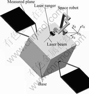
Fig. 1 Self-calibration sketch of space robot
2.3 Distance model
As shown in Fig. 2, the configuration of the calibrated 6-DOF space robot is similar to the PUMA robot. Frame ��t:ot-xtytzt represents the tool frame of the space robot, and it can be chosen arbitrarily. So, for convenience, we choose the laser ranger frame fixed on the end-effector as the tool frame, namely the origin ot is located in the starting point ps of the laser beam and the direction zt is the same as the laser beam. This process is conductive to removing some unnecessary intermediate links, since it does not need to calibrate the transformation from the tool frame to the laser ranger frame.

Fig. 2 Link coordinate frames of space robot
According to Eq. (5) and the above definition of the laser ranger frame, it is easy to know that ps with respect to the base frame ��0 equals to the translational vector pn.
Similarly, the laser beam unit vector bl with respect to the base frame ��0 is represented as
 (6)
(6)
Suppose that the measured plane equation with respect to the base frame is
nlp+f=0 (7)
where nl=(nlx, nly, nlz), is the unit normal vector of the measured plane, and its positive direction can be chosen arbitrarily. Here nlz is given a positive value. Vector p denotes the coordinate vector (px, py, pz) of the arbitrary point in the plane, and f is a known scalar. If the laser beam vector bl intersects the measured plane at the point pj, according to the relation of the vectors, pj can be written as
pj=ps+hbl (8)
where h denotes the distance from the starting point ps of the laser beam to the intersection point pj. It is known that pj also meets Eq. (7). Substituting Eq. (8) into Eq. (7), h can be given as
![]() (9)
(9)
2.4 Distance error
The distance h from Eq. (9) is an estimated value using the nominal geometric parameters of the space robot and the nominal plane equation. As stated previously, these geometric parameters on space orbit will vary with temperature environment. The geometrical errors occurring in link i can be respectively written as ����i, ��di, ��ai, ����i and ����i. If the real parameters of link i are respectively assumed as ![]() ,
, ![]() ,
, ![]() ,
, ![]() and
and ![]() , then the following equations can be given.
, then the following equations can be given.
 (10)
(10)
Therefore, the distance error ?h caused by the parameter errors can be written as
?h=h(��r, dr, ar, ��r, ��r)-h(��, d, a, ��, ��)=hr-h (11)
where hr denotes the real distance; ![]()
![]() In terms of Eq. (11), the optimized cost function H using differential evolution (DE) can be expressed as
In terms of Eq. (11), the optimized cost function H using differential evolution (DE) can be expressed as
![]() (12)
(12)
where m denotes the number of calibration configurations, and it is larger than the number of the identified geometrical parameters.
3 Geometric parameter identification by improved differential evolution
3.1 Independent geometric parameters
A complete calibration model consists of a certain number of independent geometric parameters. If the parameters exceed the scope, they will be relative; contrarily, if they are fewer than that, the model will be incomplete. EVERETT et al [21] gave the following formula of independent parameters of the robot as
C=2R+2P+6 (13)
where C denotes the number of the independent geometric parameters, R represents that of the revolved joints, and P is that of the translational joints. According to Eq. (13), the space robot shown in Fig. 2 should have 30 identifiable parameters. However, different from a laser tracker that can measure the six-dimensional pose of the robot, the laser ranger only measures the distance from the origin of the laser ranger frame to the target point. Obviously, an equidistant rotation of the end effector pointing to the target point creates no significance to the output of the laser ranger, which means to lose three constraints and cause three unidentifiable parameters. In addition, a distance equation only constrains one of the three coordinates of the origin of the laser ranger frame, while the other two coordinates are free. So, using the laser ranger, there are 25 identifiable geometric parameters for the space robot at most. Although the measurement method leads to the incomplete calibration model, its negative effect is minor, because for a space robot used to capture a space target it is unnecessary to calibrate the transformation matrix from the fixing frame to the base frame, that is, the six geometric parameters can be omitted.
3.2 Improved differential evolution algorithm
Similar to genetic algorithm, DE was also a kind of global evolutionary algorithm, presented by Storn and Price in 1995, and DE had been proven to be one of the best evolutionary algorithms. Differential evolution (DE) is encoded by real number, whose initial populations are composed of Np, D-dimensional real-valued parameter vectors. It has three operators: mutation, crossover and selection. Among them, mutation is the most original, in which new parameter vectors are created by adding the weighed difference between the two population vectors chosen randomly to the third vector as
![]() (14)
(14)
where ![]() denotes the i-th mutated vector;
denotes the i-th mutated vector; ![]()
![]() and
and ![]() represent the different parameter vectors chosen randomly in the t-th generation population; F
represent the different parameter vectors chosen randomly in the t-th generation population; F![]() (0, 2] is the scaling factor of the difference. Here, parameter i differs from a, b and c.
(0, 2] is the scaling factor of the difference. Here, parameter i differs from a, b and c.
In fact, the classical DE mutation still includes another strategy
![]() (15)
(15)
where ![]() is the best parameter vector in the current population. The strategy is generally called as DE/best/1, while the former is addressed as DE/rand/1. However, it is found in the simulation that DE/rand/1 excessively lays emphasis on the diversity of the created individual while convergence is inferior, so the desired optimization level is difficult to be gained. At the same time, DE/best/1 makes the best parameter vector in the population become the search center, which limits the diversity of the created individual and causes that optimization is very fast initially but easily gets into local minima later. Accordingly, a new tradeoff strategy is proposed in this work as
is the best parameter vector in the current population. The strategy is generally called as DE/best/1, while the former is addressed as DE/rand/1. However, it is found in the simulation that DE/rand/1 excessively lays emphasis on the diversity of the created individual while convergence is inferior, so the desired optimization level is difficult to be gained. At the same time, DE/best/1 makes the best parameter vector in the population become the search center, which limits the diversity of the created individual and causes that optimization is very fast initially but easily gets into local minima later. Accordingly, a new tradeoff strategy is proposed in this work as
![]() (16)
(16)
In spite of a small change, the optimization effect of DE has a significant improvement, which has been proved in the simulation later.
After mutation of each parameter vector, the non-uniform crossover with a crossover constant CR![]() [0, 1] between the mutated vector
[0, 1] between the mutated vector ![]() and the target vector xi is used to create the trial vector vi. Its j-th component vij is represented as
and the target vector xi is used to create the trial vector vi. Its j-th component vij is represented as
![]() (17)
(17)
where rand(j) is a uniformly distributed random number in the range of [0, 1]. The above equation shows that CR is a crossover probability that controls the components of trial vector. If CR is larger, the mutated vector occupies more trial vector. If CR=1, the trial vector vi equals ![]()
At last, the selection is carried out for reproduction. Differential evolution uses a tournament mechanism to make the trial vector compete against its target vector. If the cost function value of trial vector is smaller than that of target vector, it will survive to the next generation, and vice versa. The selection function is given as
![]() (18)
(18)
3.3 Parameter identification process based on improved DE
The improved DE is used for geometric parameter identification of space robot. As stated previously, DE has few parameters (F and CR), and is easy to program and solve the complicated optimization problem. The parameter vector x attached to the population is determined as
![]()
![]() (19)
(19)
Attentively, the two of nlx, nly and nlz in Eq. (7) are independent, and here ?nlx and ?nlz are chosen as the geometric parameters to identify. The identification process is as follows:
Step 1: Give initial values to DE parameters, for example, the population size Np, the crossover probability CR, the scaling factor F, the maximum number of generations G and the stopping criteria V;
Step 2: Give the constrained scopes of the identified parameters;
Step 3: Set i=1 and generate an initial population (Np��D) randomly in the constrained scopes;
Step 4: Calculate the cost function values of the parameter vectors in the population, and if meet H��V, go to Step 9;
Step 5: Using Eq. (16) mutate each parameter vector of the current population by randomly choosing three different members in the population;
Step 6: Using Eq. (17) create the crossover trial vectors;
Step 7: Make the trial vector compete against its target vector by comparing their cost function values according to Eq. (12), and the winning parameter vector will succeed to the next generation;
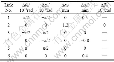
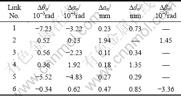
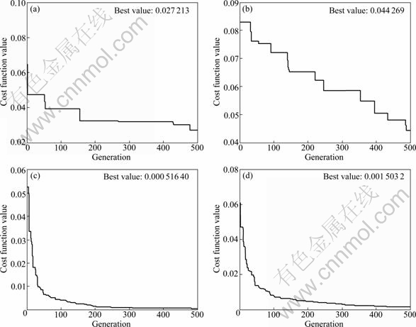
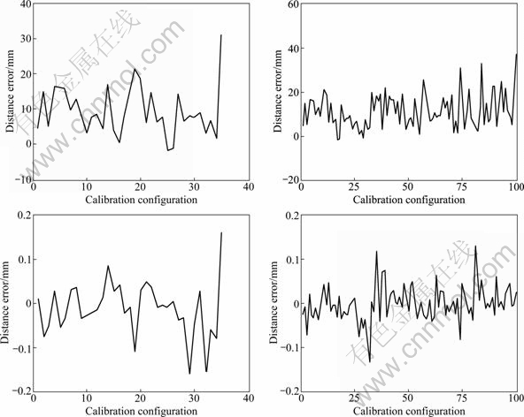
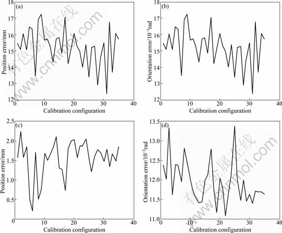
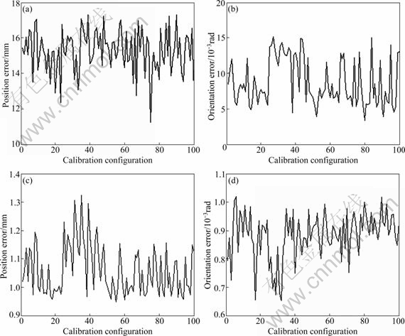
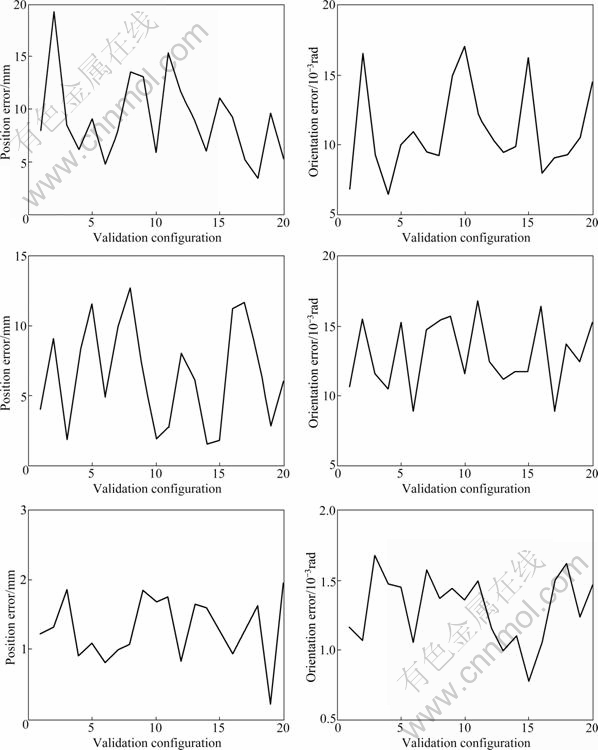
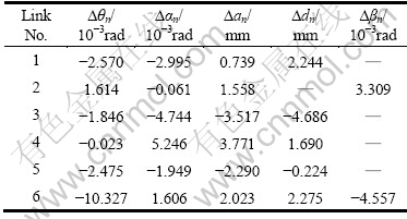
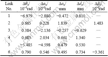
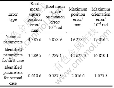
Step 8: i=i+1, if i Step 9: End the identification and obtain the optimal parameter vector. 4 Self-calibration simulation 4.1 Measurement noise There are usually some errors in the distance values measured by the laser ranger, which will create disadvantageous effect on self-calibration of space robot. In order to simulate the real case, measurement noise should be added to the error model (Eq. (11)) so as to make the calibration results more actual and effective. Here, it is assumed that distance measurement noise follows a normal distribution with zero mean and standard deviation of 0.2 mm. Because calibration configuration distance measurements are repeated many times to reduce disturbance of stochastic measurement noise, their mean is evaluated, and it is given to the calibration model as the measurement value in the calibration configuration. Of course, it is not enough that measurement noise is filtered only through the average filter. On the other hand, more redundant calibration configurations are used to calibrate the space robot to decrease disturbance of noise. The measurement value hc of the laser ranger can be simply written as hc=hr+�� (20) where �� is measurement noise. The distance error ?hc between the measurement value and the estimated one with the nominal geometric parameters can be written as ?hc=hc-h=?h+�� (21) Therefore, the cost function (Eq. (12)) optimized by DE can be modified as follows: 4.2 Generation of distance error Since self-calibration of space robot is carried out through simulation, the distance measurement values need to be simulated. Here, the generation process of the distance errors is described as follows: Step 1: Input all sets of calibration configurations, the nominal geometric parameters and the real geometric parameters of space robot; Step 2: Calculate the estimated distance h with the nominal geometric parameters; Step 3: Calculate the real distance hr with the real geometric parameters; Step 4: Generate the distance error ?h by subtracting the estimated distance from the real one; Step 5: Create n repeated measurement errors according to the above normal distribution and evaluate their mean; Step 6: Add the mean to the above distance error ?h, so ?hc is obtained. 4.3 Initial condition The nominal geometric parameters of space robot are listed in Table 1 and its pre-set geometric parameter errors are listed in Table 2. Table 1 Nominal geometric parameters of space robot Table 2 Pre-set geometric parameter errors Besides, the measured plane equation is chosen as y+4.6z-0.69=0 (23) Noticeably, as shown in Fig. 2, it cannot be chosen such the form as z+f=0, or it will make three geometric parameters unidentifiable, namely ��1, a1 and d3. Obviously, if the measured plane is perpendicular to axis z0, the three parameters will make no difference to the distance from the starting point of the laser beam to the intersecting point in the measured plane, which will result in incompleteness of the calibration model. As stated previously, the factors of the plane equation will also vary with the temperature change on orbit, and here the pre-set errors of nlx and nlz are respectively given as 0.005 and 0.01. Besides, the parameters of DE are assumed as Np=150, CR=0.9, F=0.6, G=500, V=0.000 1 (24) 4.4 Simulation result Self-calibration of space robot based on the improved DE is verified through simulation. Here, 100 calibration configurations have been chosen where the joint configurations of space robot are non-singular, and the two cases have been simulated, that is, 35 configurations, 10 repetitions, and 100 configurations, 10 repetitions. Here, the number of calibration configurations represents the configurations joining in space robot self-calibration, and the number of repeated measurements denotes the repetitions for a certain calibration configuration. Besides, a set of independent validation configurations (about 20 configurations) distributed in the whole workspace of space robot are selected to verify the calibration effect. In nature, robot calibration is a fit for the measurement data in the calibration configurations, so the extra validation configurations are necessary. Firstly, we compare the three optimization strategies of DE, DE/rand/1, DE/best/1 and tradeoff strategy presented in this work. Figures 3(a), (b) and (c) show respectively the cost function curves obtained with the above three strategies for the first case, and Fig. 3(d) shows the cost function curve obtained with the third strategy for the second case. By comparing their best values, it is easy to see that optimization efficiency of the first two classical strategies is far lower than that of the third strategy, so the improved DE has a significant progress. Besides, cost function values in Figs. 3(c) and (d) decline steeply in the beginning, then turn gentle little by little, at last end with the stopping criteria (500 iterations), which shows that the improved DE is characterized by stability and rapidity in spite of disturbance of larger measurement noise. Figures 4 (a) and (b) respectively denote the curves of the distance errors for the first and second cases in the calibration configurations before the calibration, and correspondingly, Figs. 4(c) and (d) present those after calibration. It is easy to find that calibration makes the maximum distance errors in the calibration configurations reduced from more than 30 mm to less than 0.2 mm for the first and second cases. This shows that after parameter correction the distance estimated with the identified parameters highly approaches to the real distance, so it is a very good fit for the distance measurement values. Figures 5 (a) and (b) show respectively the curves of the position and orientation errors before calibration in the calibration configurations for the first case; correspondingly, Figs. 5(c) and (d) show those after calibration. Similarly, Figs. 6(a), (b), (c) and (d) are for the second case. In nature, robot calibration is a fit for measurement data in the calibration configurations, and beyond them a discount of pose accuracy is inevitable. So, a comparison of position and orientation errors in the independent validation configurations needs to be shown. Figures 7(a) and (b) show respectively the curves of the position and orientation errors before calibration in the validation configurations; correspondingly, Figs. 7(c) and (d) show those after calibration with the identified geometrical parameters for the first case, and Figs. 7(e) and (f) are for the second case. It is easy to see that after calibration pose accuracy of the space robot has an authentic improvement. Comparatively, pose accuracy in the calibration configurations is superior to that in the validation configuration, which is consistent with our usual understanding. Fig. 3 Variation of cost function values: (a) DE/rand/1; (b) DE/best/1; (c) Tradeoff strategy; (d) Tradeoff strategy for second case Fig. 4 Distance errors before and after calibration: (a) First case before calibration; (b) Second case before calibration; (c) First case after calibration; (d) Second case after calibration Fig. 5 Pose errors before and after calibration in calibration configurations for first case: (a) Position error before calibration; (b) Orientation error before calibration; (c) Position error after calibration; (d) Orientation error after calibration Fig. 6 Pose errors before and after calibration in calibration configurations for second case: (a) Position error before calibration; (b) Orientation error before calibration; (c) Position error after calibration; (d) Orientation error after calibration Tables 3 and 4 give the identified geometric parameter errors of the space robot for the first and second cases, respectively. Table 5 gives a statistical comparison of position and orientation errors estimated respectively with the nominal and identified parameters in the validation configurations. Here, all position and Fig. 7 Pose errors before and after calibration in validation configurations: (a) Position error before calibration; (b) Orientation error before calibration; (c) Position error obtained with identified geometrical parameters for first case; (d) Orientation error obtained with identified geometrical parameters for first case; (e) Position error obtained with identified geometrical parameters for second case; (f) Orientation error obtained with identified geometrical parameters for second case orientation errors are the resultant errors of the three components of position or orientation vectors. Attentively, in principle, orientation errors cannot be synthesized because of mutual dependence of three components of an orientation vector, but here they are a tiny magnitude and can be approximated to be independent with each other. According to Table 5, it can be seen that after calibration pose accuracy of space robot in the validation configurations for the second case has a greater improvement than for the first case, which means that the magnitude of the redundant calibration configurations influences calibration results in a certain degree. More configurations embody more global characteristics, because choice of the configurations is more extensive. Besides, they can weaken unfavorable influence of measurement noise. If more calibration configurations are added, better results can be expected. Table 3 Identified geometric parameter errors of space robot for first case Table 4 Identified geometric parameter errors of space robot for second case Table 5 Pose error comparison after calibration in validation configurations 5 Conclusions 1) To overcome the influence of extreme space environment on pose accuracy of space robot, based on the improved differential evolution, a self-calibration method of the space robot whose end effector is attached to a laser ranger is developed. It is very simple (only using a laser ranger and a declining plane), and easy to carry out. 2) Location of the measured plane is important. If it is improper, it probably makes a part of geometrical parameters unidentifiable. 3) The magnitude of the calibration configurations makes a greater difference to the calibration results, because it can care for entire work space of the robot and at the same time it plays a role in filtering. 4) Classical differential evolution is improved by changing the mutation algorithm, which makes it preserve the diversity and rapidity, so increases its optimization efficiency. However, the self-calibration method proposed in this work is still a static compensation for temperature. So, the future work is to develop a self-adaptive dynamic compensation method. References [1] BEYER L, WULFSBERG J. Practical robot calibration with rosy [J]. Robotica, 2004, 22(5): 505-512. [2] SUN Y, HOLLERBACH J M. Active robot calibration algorithm [C]// Proceedings of ICRA 2008 IEEE International Conference on Robotics and Automation. Pasadena, 2008: 1276-1281. [3] KANG S H, PRYOR M W, TESAR D. Kinematic model and metrology system for modular robot calibration [C]// Proceedings of ICRA 2004 IEEE International Conference on Robotics and Automation. Barcelona, Spain, 2004: 2894-2899. [4] NEWMAN W S, BIRKHIMER C E, HORNING R J, WILKEY A T. Calibration of a Motoman P8 robot based on laser tracking [C]// Proceedings of the IEEE International Conference on Robotics and Automation. San Francisco, USA, 2000: 3597-3602. [5] LIU Y, SHEN Y T, XI X. Rapid robot/workcell calibration using line-based approach [C]// Proceedings of the 4th IEEE Conf on Automation Science and Engineering. Washington DC, USA, 2008: 510-515. [6] ZHUANG H, ROTH Z S, WANG K. Robot calibration by mobile camera system [J]. Robotic Systems, 1994, 11(3): 155-168. [7] ALICI G, SHIRINZADEH B. A systematic technique to estimate positioning errors for robot accuracy improvement using laser interferometry based sensing [J]. Mechanism and Machine Theory, 2005, 40(8): 879-906. [8] GONG C H, YUAN J X, NI J. Nongeometric error identification and compensation for robotic system by inverse calibration [J]. International Journal of Machine Tools & Manufacture, 2000, 40(14): 2119-2137. [9] LIGHTCAP C, HAMNER S, SCHMITZ T, BANKS S. Improved positioning accuracy of the PA10-6CE robot with geometric and flexibility calibration [J]. IEEE Transactions on Robotics, 2008, 24(2): 452-456. [10] RADKHAH K, HEMKER T, STRYK O. A novel self-calibration method for industrial robots incorporating geometric and non-geometric effects [C]// Proceedings of the IEEE International Conference on Mechatronics and Automation. Takamatsu, Japan, 2008: 864-869. [11] DROUET P, DUBOWSKY S, ZEGHLOUL S, MAVROIDIS C. Compensation of geometric and elastic errors in large manipulators with an application to a high accuracy medical system [J]. Robotica, 2002, 20(3): 341-352. [12] JANG J H, KIM S H, KWAK Y K. Calibration of geometric and nongeometric errors of an industrial robot [J]. Robotica, 2001, 19(3): 311-321. [13] ZHONG X L, LEWIS J, N-NAGY F L. Inverse robot calibration using artificial neural networks [J]. Engineering Applications of Artificial Intelligence, 1996, 9(1): 83-93. [14] VICENTE R, CARME T. Self-calibration of a space robot [J]. IEEE Trans on Neural Network, 1997, 8(4): 951-962. [15] DOLINSKY J U, JENKINSON I D, COLQUHOUN G J. Application of genetic programming to the calibration of industrial robots [J]. Computers in Industry, 2007, 58(3): 255-264. [16] ALICI G, JAGIELSKI R, et al. Prediction of geometric errors of robot manipulators with Particle Swarm Optimisation method [J]. Robotics and Autonomous Systems, 2006, 54: 956-966. [17] HIRZINGER G, LANDZETTEL K, ADZETTEL K, BRUNNER B, FISCHER M, PREUSCHE C, REINTSEMA D, ALBU-SCHAFFER A, SCHREIBER G, STEINMTZ B-M. DLR��s robotics technologies for on-orbit servicing [J]. Advanced Robotics, 2004, 18(2): 142-144. [18] HIRZINGER G, BRUNNER B, DIETRICH J, HEIDL J. Sensor- based space robotics-ROTEX and its telerobotic featuresm [J]. IEEE Trans On Robotics and Automation 1993, 9(5): 649-663. [19] GATLA C S, LUMIA R, WOOD J, STARR G. Calibration of industrial robots by magnifying errors on a distant plane [C]// Proceedings of the IEEE Int Conf on Intelligent Robots and Systems. San Diego, 2007: 3834-3841. [20] VEITSCHEGGER W K, WU C H. Robot accuracy analysis based on kinematics [J]. IEEE Transactions on Robotics and Automation, 1986, 2(3): 171-180. [21] EVERETT L, DRIELS M, MOORING B. Kinematic modeling for robot calibration [C]// Proceedings of the IEEE Int Conf on Robotics and Automation. San Francisco, 1987: 183-190. (Edited by DENG L��-xiang) Foundation item: Projects(60775049, 60805033) supported by National Natural Science Foundation of China; Project(2007AA704317) supported by the National High Technology Research and Development Program of China Received date: 2011-01-11; Accepted date: 2011-03-24 Corresponding author: LIU Yu, Associate Professor, PhD; Tel: +86-451-86402330; E-mail: lyu11@hit.edu.cn![]() (22)
(22)
Abstract: Due to the intense vibration during launching and rigorous orbital temperature environment, the kinematic parameters of space robot may be largely deviated from their nominal parameters. The disparity will cause the real pose (including position and orientation) of the end effector not to match the desired one, and further hinder the space robot from performing the scheduled mission. To improve pose accuracy of space robot, a new self-calibration method using the distance measurement provided by a laser-ranger fixed on the end-effector is proposed. A distance-measurement model of the space robot is built according to the distance from the starting point of the laser beam to the intersection point at the declining plane. Based on the model, the cost function about the pose error is derived. The kinematic calibration is transferred to a non-linear system optimization problem, which is solved by the improved differential evolution (DE) algorithm. A six-degree of freedom (6-DOF) robot is used as a practical simulation example, and the simulation results show: 1) A significant improvement of pose accuracy of space robot can be obtained by distance measurement only; 2) Search efficiency is increased by improved DE; 3) More calibration configurations may make calibration results better.
