

J. Cent. South Univ. (2020) 27: 1334-1350
DOI: https://doi.org/10.1007/s11771-020-4370-6

Numerical investigation of influence of pantograph parameters and train length on aerodynamic drag of high-speed train
SUN Zhi-kun(��־��)1, WANG Tian-tian(������)1, 2, WU Fan(�鷰)1
1. School of Traffic & Transportation Engineering, Central South University, Changsha 410075, China;
2. College of Mechanical and Vehicle Engineering, Hunan University, Changsha 410082, China
 Central South University Press and Springer-Verlag GmbH Germany, part of Springer Nature 2020
Abstract:
This study investigates the influence of different pantograph parameters and train length on the aerodynamic drag of high-speed train by the delayed detached eddy simulation (DDES) method. The train geometry considered is the high-speed train with pantographs, and the different versions have 3, 5, 8, 10, 12, 16 and 17 cars. The numerical results are verified by the wind tunnel test with 3.6% difference. The influences of the number of cars and the position, quantity and configuration of pantographs on flow field around high-speed train and wake vortices are analyzed. The aerodynamic drag of middle cars gradually decreases along the flow direction. The aerodynamic drag of pantographs decreases with its backward shift, and that of the first pantograph decreases significantly. As the number of pantographs increases, its effect on the aerodynamic drag decrease of rear cars is more significant. The engineering application equation for the aerodynamic drag of high-speed train with pantographs is proposed. For the 10-car and 17-car train, the differences of total aerodynamic drag between the equation and the simulation results are 1.2% and 0.4%, respectively. The equation generalized in this study could well guide the design phase of high-speed train.
Key words:
high-speed train; pantograph; train length; aerodynamic drag��
Cite this article as:
SUN Zhi-kun, WANG Tian-tian, WU Fan. Numerical investigation of influence of pantograph parameters and train length on aerodynamic drag of high-speed train [J]. Journal of Central South University, 2020, 27(4): 1334-1350.
DOI:https://dx.doi.org/https://doi.org/10.1007/s11771-020-4370-61 Introduction
When the speed of high-speed train reaches 350 km/h, aerodynamic drag accounts for about 75% of the total train resistance [1]. The aerodynamic drag of high-speed train is needed to be accurately evaluated [2]. The pantograph parameters and train length have a significant influence on the train aerodynamic drag. In order to improve the transportation efficiency, the possible methods are to increase the number of cars or use double-unit train. Compared with single-unit train, double-unit train causes higher slipstream velocity, which challenges the safety of passengers and workers at the platform edge [3, 4], and generates noise pollution to the surrounding environment, which leads to the potential hearing loss in train drivers [5, 6]. The use of double-unit train will increase the train aerodynamic drag and adversely affect the electrical facilities [7, 8]. Therefore, the increase of cars of single-unit train is generally used for the improvement of transport capacity.
Experimental methods on aerodynamic drag of high-speed train mainly include field experiment, model test and numerical simulation [9, 10]. Field experiment can reflect the actual operation of high-speed train [11], but the cost is huge. Model test, which includes wind tunnel test and moving model test, is widely used for high-speed train experimental research [12-14]. Due to the limitation of length of test section, 2 or 3 cars are generally used for the model test [15-17], while trains with long length is generally studied by CFD simulations. Reynolds-averaged Navier-Stokes simulation (RANS), large eddy simulation (LES) and detached eddy simulation (DES) are widely used for the simulation of turbulent flow around high-speed train [18-21]. LI et al [22] investigated the effect of RANS turbulence model on aerodynamic behavior of trains in crosswind. JI et al [23] studied the calculation grid and turbulence model for numerical simulating pressure fluctuations in high-speed train tunnel. WANG et al [24] researched the influence of enlarged section parameters on pressure transients of high-speed train passing through a tunnel. RANS is difficult to predict the separated flows in the wake region [25]. LES requires extremely high computational costs [26, 27]. The aerodynamic performance of high-speed train running in the open air is generally calculated by DES [28, 29]. Compared with LES, DES effectively reduces the computational cost for high Reynolds number situations. However, DES has the significant weaknesses of the modeled-stress depletion and the grid induced separation [30]. Delayed-DES (DDES) based on DES is introduced to improve the above deficiencies [31], which performs well when capturing small flow structures periodically generated in the shear layer [32].
The aerodynamic study on train length is mainly investigated on the influence of aerodynamic performance, slipstream, boundary layer and wake development. In the current researches, train with over 8 cars is rarely studied. And special structures such as pantographs, which have significant effects on the flow field around the train, are simplified. HUANG et al [33] studied the aerodynamic drag of each car in the 2-6 car situations through wind tunnel test. The drag coefficient of the head and the tail car is slightly changed when the number of cars is larger than 3. MULD et al [34] simulated the flow around train with different numbers of cars (2, 3, and 4) by DES, and the dominant flow structure in the wake is the same for all three cases. However, the frequency of this structure decreases while the boundary-layer thickness is increasing for these train configurations. BELL et al [35] carried out a moving model test to study the effects of reduced length to height ratio on the wake and tail surface pressure of a high-speed train. A similar conclusion with the results of Ref. [34] is obtained, that is, the key features of the wake topology are consistent regardless of the length to height ratio. JIA et al [36] used DDES to simulate the effects of train length on the boundary layer, wake, surface pressure, aerodynamic drag and frictional resistance of high-speed train without pantographs. Four train configurations are employed, including 3, 4, 5 and 8 cars. NIU et al [37] adopted DDES to study the lateral stability of high-speed train of different lengths under crosswind with or without windbreaks. In this manuscript, the DDES method is adopted to investigate the influence of high-speed train pantograph parameters and train length on aerodynamic drag. The numerical simulation method is proposed according to the wind tunnel test. The influence of the position, quantity and configuration of the pantograph on the flow field structure is analyzed. The differences of the pantograph aerodynamic drag at different positions are significant, which has a significant impact on pantograph strength design. An engineering application equation is proposed, which can effectively estimate the aerodynamic drag of high-speed train with different pantograph parameters and train length. The equation will be of good guiding significance for the design process of high-speed train.
2 Numerical simulation
2.1 Computational model
In this study, a certain type of 1:8 scaled high-speed train is employed for numerical simulation. The configurations of trains with different length and pantograph parameters are illustrated in Figure 1(a). H represents the height of train model, which is 0.515 m. Each configuration consists of the head car, N middle cars and the tail car. N is set as 1, 3, 6, 8, 10, 14 and 15, respectively. All cars are numbered sequentially from the head car. The pantographs, bogies and windshields are modeled in every configuration for better flow field simulation. Except for the train length and pantograph configuration, the other geometries of the train model keep consistent. The raised and unraised pantographs of the train are shown in Figures 1(b) and (c). For middle car, the positions of raised and unraised pantographs, windshields and bogies are shown in Figure 1(d), respectively. The number of cars and the position, quantity and configuration of pantographs in each case are listed in Table 1. The Case 4 in Table 1 is an 8-car group without the unraised pantograph on the third car. Ltr represents the length of the train. URP and RP are the unraised and raised pantograph, respectively. Position is the serial numbers of the cars where the pantograph is located.
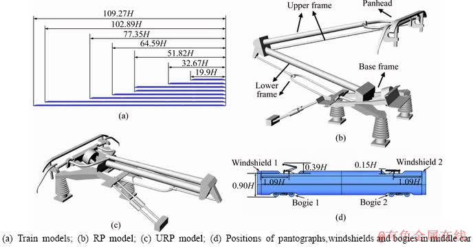
Figure 1 Computational models:
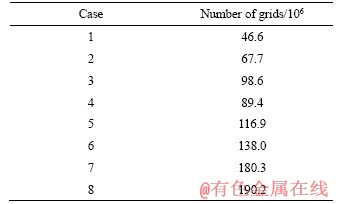
Table 1 Computational cases

2.2 Computational domain and boundary conditions
Figure 2 shows the computational domain and boundary conditions for the numerical simulation in this study. The upstream distance between the inlet and the train nose is 20H. The downstream distance Xd (between the exit and the tail) should be as long as possible to ensure the full development of the wake and Xd is selected as 1.5 Ltr. The width of the domain is 10H, and the height is 5H. The distance between the bottom of the wheel and the ground is 0.05H. The inlet is set as velocity inlet boundary, and the velocity is set to be equivalent to that of the train speed, i.e., 350 km/h. The outlet is set as pressure outlet boundary. The upper surface and both sides are set as symmetry boundary. The ground is set as moving no-slip wall to simulate the relative movement between the train and the ground. The moving speed of the ground is 350 km/h. The train surface is defined as no-slip wall.
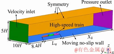
Figure 2 Computational domain and boundary conditions
2.3 Computational mesh
As is shown in Figure 3, the complex pantograph and bogie areas are discretized with unstructured grid, and rest of the domain is discretized with structured grid. In the simulations of this paper, the thickness of the first layer of boundary grid is 0.125 mm. The size of grid on surface of train nose, bogie and pantograph are all about 2.5 mm, while that of train body is approximately 6.25 mm. In order to simulate the formation and shedding of turbulence in the wake region for accurately simulating aerodynamic drag of the tail car, the mesh of train wake is relatively dense. The numbers of mesh cells corresponding to different train configurations are shown in Table 2. The range of y+ in this study is basically between 32 and 83.
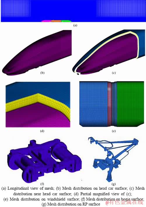
Figure 3 Computational mesh:
2.4 Numerical method
The commercial CFD software ANSYS Fluent is employed for the numerical simulations in this study. Since the y+ range of the computational mesh is between 32 and 83, the DDES method based on a realizable k-�� turbulence model is adopted in this paper. The incompressible flow is used because the Mach number is less than 0.3 in the calculations. SIMPLEC (semi-implicit method for pressure- linked equations consistent) algorithm is employed for solving the discretized equations. The standard discretization scheme is used for the pressure term, and the second-order upwind discretization scheme for the momentum term, turbulent kinetic energy term and turbulent dissipation rate term. The computational time step ��t is set as 0.1 ms. In all cases, the calculation time Tc=3Ld/Vt, where Ld is the length of computational domain along the flow direction and Vt is the train speed, which is 97.222 m/s. The sampling time Ts=2/3Tc, and the sampling starts at t=1/3Tc. The number of inner iterations is 30. Based on the train speed and the value of H, the Reynolds number of the numerical simulations is approximately 3.34��106, which is greater than 2.5��105 [38]. The flow is fully turbulent so that the aerodynamic coefficients are believed to be Reynolds number independent [38]. The change of Reynolds number will not affect the results [40-42].
Table 2 Numbers of computational grids in different cases
3 Validation
3.1 Brief introduction of wind tunnel test
A 1:8 scale 3-car train model is used in the wind tunnel test, which is the same as the computational model employed in this paper. The test section is shown in Figure 4(a). The train model is placed in the test section measuring 15 m (Length)��8 m (Width)��6 m (Height), where the wind speed ranges from 20 to 100 m/s. The test wind speed is 65 m/s, the corresponding Reynolds number is 5.7��106. The floor and aerodynamic balances used in the wind tunnel test are dedicated for trains .
As can be seen from Figure 4(a), the train model is installed on a platform at a certain height from the ground, which avoids the influence of the ground boundary layer of the test section on the test results. The platform is formed by splicing 4 boards. The structure and specific dimensions of the platform are shown in Figure 4(b). The upper surface of the platform is 1.06 m away from the ground of the wind tunnel. In the middle of the platform is a rotating disk. The center of the rotating disk is 7.83 m from the front edge of the platform and 7.33 m from the rear edge. The front and rear edges of the platform are processed to be streamlined to reduce the disturbance to the airflow. The effect of the floor boundary layer is reduced by the pumping action of the gap. The effective size of the test section is 15.16 m long, 8 m wide, 4.94 m high, and the effective cross-sectional area is 39.20 m2. A 1:8 scaled subgrade model with a length of 27.18H is placed on the platform, and the track model with a length of 26.45H is located on the subgrade. In the center of spanwise direction, the train model with a length of 19.42H is located on the track. The models used in the wind tunnel test are shown in Figure 5(a), the train model retains the details such as the pantographs, bogies, and windshields. Three six-component box-type force balances are set to measure the drag forces of the three cars. The DSM3400 electronic pressure scanning valve system produced by Scanivalve is used to measure the train surface pressure. The measuring range is ��1 Psi (approx. 6895 Pa) with the accuracy of �� 0.08% FS.
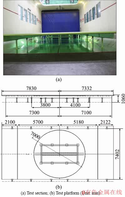
Figure 4 Test section and platform of the wind tunnel:
The computational mesh and numerical method adopted in this paper are validated by the wind tunnel experiment. The train model used in the numerical validation, as shown in Figure 5(b), is consistent with the test model, including the same scale and details (pantograph, bogies, gaps etc.). The computational domain has the same scale as the test section, with platform, subgrade and track at the same location. The ground is set as a stationary no-slip wall, consistent with the wind tunnel test. The computational mesh is generated in the same scheme as the mesh in Section 2.3.
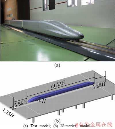
Figure 5 1:8 scaled model used in wind tunnel test and numerical validation:
3.2 Comparison and analysis
According to the CEN European Standard [43, 44], the aerodynamic pressure and drag are dimensionless, which are defined as follows:
 (1)
(1)
 (2)
(2)
where Cd is the aerodynamic drag coefficient. Fd is the aerodynamic drag. The incoming flow density �� is 1.225 kg/m3. V is the test wind speed, the value of which is 65 m/s. S is the reference area of train model, the value of which is 0.1866 m2. Cp is the pressure coefficient on the train surface. p and p�� are the pressures on the train surface and the static pressure outside the wind tunnel, respectively.
Three computational grids for 3-car train are generated based on the experimental setup for mesh independency test. The numbers of coarse, medium and fine mesh are 106��106, 141 million, and 163 million, respectively. For comparison, the 17-car train are selected. The numbers of coarse, medium and fine mesh are 289��106, 351��106, and 401��106, respectively. Table 3 indicates the difference between the numerical simulation and the test. The results of the coarse mesh differ greatly from the experimental ones, while the difference of the medium mesh is close to that of the fine mesh, which are all within 5%. It can be concluded that the medium grid basically meets the requirements of numerical simulation. The mesh of the cases in Table 1 is constructed with a medium grid generation strategy.
Table 3 Difference of Cd obtained from numerical simulation and test
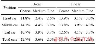
Figure 6 compares the pressure coefficient distribution along horizontal line at the height of z=0.125 m and the longitudinal symmetry line over the upper surface of head and tail car between the simulation and test results. x/H indicates the horizontal distance from the center of train model normalized by H. The surface pressure distribution in the numerical simulation shows good agreement with the experimental results. In conclusion, the overall agreement in aerodynamic forces and pressure validates that the computational grid and methodology adopted in this paper are sufficient to achieve accurate numerical result.
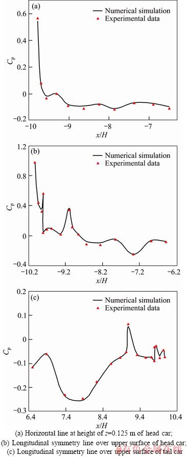
Figure 6 Comparison of surface pressure on head and tail car between test results and numerical results of medium mesh:
4 Results and discussion
4.1 Influence of pantographs
Table 4 shows Cd of each car in different computational cases. HC and TC represent the head and tail car, respectively. MC1-MC15 represent the first to fifteenth middle car, respectively. As the DDES method is adopted for numerical simulation, the aerodynamic drag analyzed in this paper is time-averaged results. The installed position and configuration of pantograph can be seen in Table 1. As shown in Table 4, Cd of head car is basically the same since the rear cars influence slightly on the upstream flow. Consequently, Cd of head car is not affected by the change of train length and pantograph parameters. Cd of tail car is affected by the pantographs and train length. Except for the 3-car and the 5-car group with pantograph on the penultimate car, the other cases have approximately the same Cd of tail car. For high-speed train with different groups, the position, quantity and configuration of pantographs have a significant influence on the aerodynamic drag, while bogies and other structures have a relatively constant influence on the aerodynamic drag. Therefore, the pantograph should be analyzed specifically.
Table 4 Cd of cars in each case
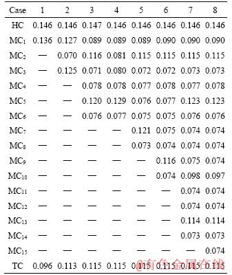
Figure 7 shows the symmetrical longitudinal section (y=0 m) of the boundary layer (represented by the black line) in the 3-car group and 8-car groups with and without URP. In this paper, Flow velocity is normalized by the velocity of incoming flow. For trains without pantographs, the thickness of boundary layer gradually increases along the train length. In these 3 cases, the pantographs are completely immersed into the boundary layer. As shown in Figure 7(a), in the RP region of the 3-car group, there are two bulges of boundary layer, one in front of the slide plate while another above the upper arm. Between the upper and lower arms is a closed curve of boundary layer. In Figure 7(b), in the URP region of the 8-car group, there is a bulge and a small closed curve of boundary layer above URP. RP of the 8-car group is surrounded by the fully turbulent flow. According to Figures 7(a) and (c), with the backward shift of pantograph along the flow direction, the boundary layer is thicker in front of RP and the low-velocity region of incoming flow is larger. The boundary layer thickness at the rear of RP of the 3-car group is much higher than URP of the 8-car group, with a larger turbulent region inside. The vortex structures at the rear of URP and RP are shown in Figure 11.
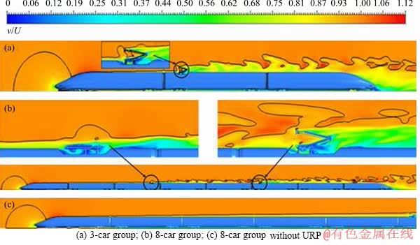
Figure 7 Symmetrical longitudinal section (y=0 m) of boundary layer:
Table 5 indicates the Cd for pantographs in each case. The first pantograph of the 5-car group and the 8-car group is unraised. The former one is placed on MC1, while the latter one is placed on MC2. Cd of the URP decreases by 0.001 due to the backward shift along the flow direction. The first pantograph of the 3-car group and 8-car group without URP are raised. The position of the latter is shifted back by the length of 4 cars compared with the former, and Cd decreases by 0.004 due to the increase of the boundary layer thickness.
Table 5 Cd of pantographs in each case

The pantograph contains many cylindrical rods. Many circular-cylinder flow structures are produced as the incoming flow pass through the first pantograph. The effect of the first pantograph on the flow field leads to the formation of a fully developed turbulence region downstream, which reduces Cd of the downstream car body and other pantographs. Compared with the RPs of 8-car group with and without URP, the incoming flow of the latter one is not affected by the front pantograph. Flow velocity and Cd of the latter one are larger as only the boundary layer develops along the car surface. In the 8-car group and the 12-car group, the first pantograph, which is unraised, is on MC2. Cd of RP decreases with the backward shift along the flow direction. The flow velocity distribution of 2 sets of pantographs in the 16-car group is shown in Figure 10. The average flow velocity after the air flows through multiple pantographs significantly reduces. Consequently, Cd of the latter set of pantographs is 0.009 lower than the former set of pantographs.
Figure 8 shows the symmetrical longitudinal section (y=0 m) of the flow velocity distribution in URP region of the 5-car group and 8-car group. Flow separation is generated by the sinking of base in Region 1, and the separated flow reattaches on the surface in Region 3. Therefore, Cd of the car body significantly increases, and that of MC2 increases by 0.035 owing to the pantograph installation, as shown in Table 6. In Region 2, when the position of pantograph is shifting back along the flow direction, the immersed height of pantograph into the boundary layer is larger. As a result, Cd of pantograph decreases. In Region 4, the separation region caused by the flow getting off the sinking base covers the rear windshield, and it leads to the reduction of Cd of Windshield 2 in Table 7.
The comparison of RP and URP on the same car is conducted to investigate the influence of the pantograph configurations on the flow field.Figure 9 shows the symmetrical longitudinal section (y=0 m) of the flow velocity distribution of MC1 in the 3-car group and the 5-car group. Due to the raised form, the windward area of RP increases. Consequently, Cd of RP and MC1 in the 5-car group is greater than Cd of URP and MC1 in the 3-car group, respectively. Compared with RP installed at the front part of car body, URP has less influence on Cd of the installed car, but significantly reduces Cd of the next car.
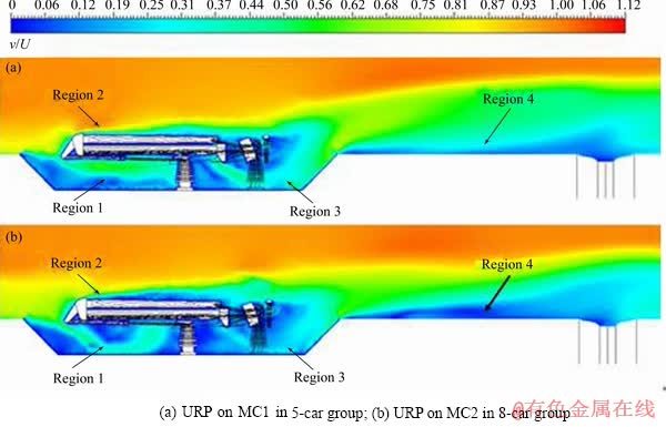
Figure 8 Symmetrical longitudinal section (y=0 m) of flow velocity distribution in URP region:
Table 6 Pressure and viscous drag coefficients of each car

Table 7 Pressure and viscous drag coefficients of different parts at MC2
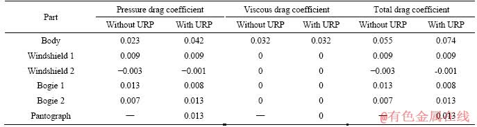
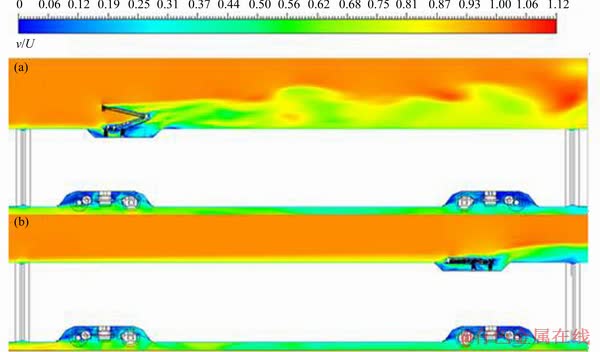
Figure 9 Symmetrical longitudinal section (y=0 m) of flow velocity distribution of MC1 in 3-car group (a) and 5-car group (b), respectively
4.2 Influence of train length
The train aerodynamic drag is affected by the pantographs and train length. The effect of train length was studied by MULD et al [34] and JIA et al [36]. For the first four middle cars in Case 4, Cd decreases as the serial number of cars increases, but the downward trend gradually slows down. Since the boundary layer thickness of the first five cars increases rapidly, the change of the pantograph position has a significant influence on Cd of cars. Except for the 3-car group and the 5-car group, all the pantographs installed on the first five cars in other cases are unraised on MC2.
The 8-car groups with and without URP are compared to analyze the effect of pantograph and train length on the aerodynamic drag of high-speed train. Table 6 gives the pressure and viscous drag coefficients of each car in 8-car groups with and without URP. As the boundary layer thickness increases along the flow direction, the viscous drag coefficient of middle cars decreases. The viscous drag occupies a larger proportion in Cd of middle cars than that in Cd of head and tail car as shown in Table 6.
The contribution of each train component to the aerodynamic drag is analyzed by comparing MC2 in the 8-car groups with and without URP. Table 7 shows the pressure and viscous drag coefficient of MC2 in these 2 cases, respectively. The viscous drag coefficient of the parts expect for body is approximated to 0 in Table 7 since the viscous drag of them is small. In addition to Cd of pantograph, the sinking base also increases the pressure drag of car body and slightly reduces the viscous drag. The flow around Windshield 1 is not affected by the structural changes of MC2, so the drag keeps consistent. It can be seen from Figure 8(b), the flow around Windshield 2 is affected by the pantograph, and the absolute value of Cd slightly decreases compared to that in the 8-car group without URP. Due to the pantograph installation, the Cd distribution of the bogie changes, but the total drag of that remains approximately consistent.
Figure 10 shows the symmetrical longitudinal section (y=0 m) of the flow velocity distribution of two sets of pantographs in the 16-car group. As shown in Figure 10(a), the first half of flow field on top of MC3 in the 8-car group with URP is still in the separation region behind URP. The flow velocity in the region is lower, so the pressure drag significantly decreases. For the train with 2 sets of pantographs, when the flow passes through the first set of pantographs, the turbulent region behind them is fully developed, and it basically covers the latter set of pantographs. Consequently, Cd of the latter set of pantographs gradually stabilizes as the position shifts backwards, and their effect on Cd of the rear car changes slightly. As shown in Table 4, Cd of car without pantograph behind the third pantograph in the 16-car and 17-car groups tends to be consistent.
The iso-surface of constant Q is used to describe the transient vortex structure. Figure 11 presents instantaneous flow structures around the train and at the train wake, visualized by Q. The influence of URP at MC2 on the instantaneous flow structures of rear cars is investigated in Figure 11(b). For Region 3 of the 8-car group without URP, except for the flow structures caused by the interaction between bogies and ground, there are only a few vortices around the upper part of car body due to the smooth car surface. Therefore, Cd of middle cars in front of RP is only affected by the development of boundary layer. In the 8-car group, a large number of small vortices are shed from URP and growing backwards. Each time passing through a pantograph, the vortices are broken into smaller structures, and accordingly Cd of middle cars is reduced as shown in Table 4.
A comparison of the vortex structures, which are caused by the pantograph and then shed from the upper edge of tail car, is conducted between the 3-car group and 8-car group. There are less but more continuous vortex structures in the 3-car group, and a periodic alternating main vortex can be seen in Region 1. However, as the number of pantographs increases, more small and complicated vortices are seen in the 8-car group. The main wake structure shed from the lower edge of train is investigated, and its change affected by the train length is analyzed. In Region 1 near the tail car, as the train length increases, the main wake structure is approximately consistent, which is consistent with the results of Ref. [34] and Ref. [35]. In Region 2 away from the tail car, the vortices at the bottom roll up and merge with the vortices generated by pantographs. Comparing to the 3-car group, the combined location of vortex structures in the 8-car group is farther.
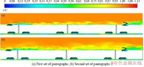
Figure 10 Symmetrical longitudinal section of flow velocity distribution of two sets of pantographs in 16-car group (y=0 m):

Figure 11 Instantaneous flow structures around train (Iso-surface of second invariant of velocity gradient Q=400, colored by static pressure ranged from -1000 to 500 Pa):
4.3 Engineering application equation
A single car is the basic unit in the design phase of high-speed train. The engineering application equation of Cd for the high-speed train with different train lengths is proposed. This equation can estimate the changes of Cd caused by different pantograph parameters and train lengths. Variations of pantographs include the configuration, quantity and position. The relationship between Cd and train length can be expressed by a fitting curve. The change of train length will not affect Cd of the head car, and Cd of the tail car is not sensitive to it except the 3-car group and 5-car group. In this paper, Cd of the head and tail car is assumed to be 0.146 and 0.115, respectively.
According to the aerodynamic drag distribution of 8-car group without URP given in Table 4, it is assumed that Cd of middle cars behind MC4 is equal to that of MC4. The Cd data of the first 15 cars is fitted by the linear equation, and the fitting curve is shown in Figure 12. For high-speed train of which the pantographs are simplified, Cds, which represents Cd of all the middle cars, is calculated in Eq. (3). x is the distance along the flow direction, which take the nose of the head car as the beginning and the end of the last middle car as the destination. x/H is greater than 6.76 (the normalized length of head car) since the equation applies to the train which contains at least one car.
 (3)
(3)
In addition to the train length, Cd of high-speed train is also affected by pantographs. As shown in Figure 10(b), when the train length is long, the rear pantographs are in the fully developed turbulent region. Cd of rear pantographs gradually stabilize as the position shifts backwards. Based on the analysis of the influence of pantograph parameters on the flow field and the Cd trend of pantographs, the scatter data of URP and RP in Table 5 is fitted by the exponential function. The drag calculations are shown in Eqs. (4) and (5). Cdr and Cdur are the aerodynamic drag coefficients of RP and URP, respectively. The destination of the distance for pantograph is defined as the center of its sinking base. Figures 13(a) and (b) present the fitting curves of Cdr and Cdur, respectively.
 (4)
(4)
 (5)
(5)
The change in Cd of car with pantograph includes Cd of the pantograph itself and the Cd change of car body caused by the sinking base. The difference of Cd between car with and without pantograph is exponentially fitted, and the drag calculation is shown in Eqs. (6) and (7). Cdrt and Cdurt are the aerodynamic drag of car with RP and URP, respectively. The destination of the distance is defined as the center of the sinking base of pantographs. The fitting curves are shown in Figures 13(c) and (d).
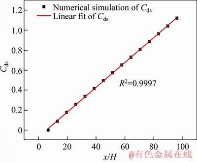
Figure 12 Fitting curve of Cds
 (6)
(6)
 (7)
(7)
It is assumed that except for the first set of pantographs, the other pantographs have the same effect on the reduction of Cd of rear cars. Based on the discussion in Sections 4.1 and 4.2, the aerodynamic drag coefficient of high-speed train with pantographs (without the head and tail cars) is shown in Eq. (8):

 (8)
(8)
where i, j and k represent the serial number of RPs, URPs and pantographs, respectively. xi and xj are the distance from the nose of head car to the number i RP and number j URP, respectively. y1 to yk-1 respectively represent the distance between the nose of head car and the first to number k-1 pantograph. yk represents the distance between the nose of head car and the end of the last middle car. l, m and n are the total number of the RPs, URPs and pantographs, respectively. �� is defined in Eq. (9):
 (9)
(9)
where Cdf and Cdr represent Cd of the front and rear car of the car with pantograph, respectively. The weakening coefficient of Cd of pantograph to the rear cars, d, is defined in Eq. (10):
 (10)
(10)
where Lcar is the middle car length, the value of which is 6.38 m. d1 is the average d of the first URP calculated from Cases 3, 6 and 7 in Table 4. Cdr used to calculate d1 is Cd of the second car at the rear of car with URP. d2 is the average d of the first RP calculated from Cases 3 and 7 in Table 4. d3 is d of the third pantograph calculated from Case 7 in Table 4. Since the first pantograph is unraised, which has a significant influence on the latter car, the constant b is introduced to correct the drag. The above coefficients in Eq. (8) are obtained based on the numerical simulations of trains with different number of cars include 3, 5, 8, 12 and 16 cars. Consequently, d1=0.0019, d2=0.0002, d3=0.0002, b=-0.0055.
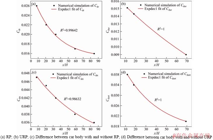
Figure 13 Fitting curves of Cd:(Expdec 1 is a single exponential fitting)
Cd of the whole train, defined as Cdw, is calculated as shown in Eq. (11):
 (11)
(11)
where CdH is Cd of the head car, and CdT is Cd of the tail car. They vary due to the change of head streamline shape and other major structures, but it can be considered that they are basically not affected by the change of train length.
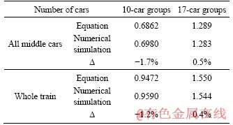
The equation is verified by the numerical results of the 10-car and 17-car groups, as shown in Table 8. �� denotes the difference of the numerical simulation results from the calculated results (based on the numerical simulation). The results obtained from the proposed equation agree well with that from the numerical simulation. Therefore, the equation can be adopted as an engineering application equation for the aerodynamic drag of high-speed train with pantographs.
Table 8 Calculated and numerical results of 10-car and 17-car groups
In Eq. (8), Cdt is only related to the train length and the configuration, quantity and position of pantographs. In this manuscript, the train length is normalized by H. Since the structure and position of bogies at each car are approximately consistent, and the influence of windshields on Cd of the whole train is slight [32, 44], it can be considered that the value of Cdt is independent of the specific train model. The proposed equations are available for the EMU with over 2 marshalling cars. From Eq. (11), it can be concluded that for different configurations of train lengths and pantograph parameters, the aerodynamic drag of high-speed train with pantographs can be estimated when that of the head and tail cars are known. For example, through the numerical calculation of the aerodynamic drag of 2-car group, the aerodynamic drag of high-speed train with different pantograph parameters and train lengths can be obtained.
5 Conclusions
In this paper, the effect of different pantograph parameters and train lengths on the aerodynamic drag of high-speed train is investigated. The difference of results between the numerical simulation and the wind tunnel test is 3.6%. The numerical simulation results of different train configurations are analyzed:
1) The viscous drag and Cd of middle cars gradually reduce along the flow direction due to the increase of boundary layer thickness.
2) Cd of pantograph decreases with its backward shift, and Cd of the first pantograph decreases significantly.
3) The pantograph and its sinking base are the main reason for the Cd increase of cars with pantograph. The complex turbulent area formed behind pantograph is the main cause of the Cd decrease of cars without pantograph.
4) The flow field around the rear car roof behind URP is in the separation region, which leads to Cd of the rear car decrease much larger than other cars without pantographs.
The maximum pantograph aerodynamic drag in this manuscript is 1800 N and the minimum is 1106 N. As a result, the difference of pantograph aerodynamic drag reaches 62.7%, which has a significant impact on pantograph strength design. The engineering application equation for the aerodynamic drag of high-speed train with pantographs is proposed, which can effectively estimate the influence of pantograph parameters and train lengths on aerodynamic drag of the EMU with over 2 marshalling cars. The equation could provide the good references for the aerodynamic design of high-speed train.
References
[1] TIAN H. Formation mechanism of aerodynamic drag of high-speed train and some reduction measures [J]. Journal of Central South University of Technology, 2009, 16(1): 166-171. DOI: https://doi.org/10.1007/ s11771-009-0028-0.
[2] SOMASCHINI C, ARGENTINI T, ROCCHI D, SCHITO P, TOMASINI G. A new methodology for the assessment of the running resistance of trains without knowing the characteristics of the track: Application to full-scale experimental data [J]. Proceedings of the Institution of Mechanical Engineers, Part F: Journal of Rail and Rapid Transit, 2018, 232(6): 1814-1827. DOI: https://doi.org/10.1177/0954409717751754.
[3] BAKER C. The flow around high speed trains [J]. Journal of Wind Engineering and Industrial Aerodynamics, 2010, 98(6, 7): 277-298. DOI: https://doi.org/10.1016/j.jweia.2009. 11.002.
[4] FLYNN D, HEMIDA H, BAKER C. On the effect of crosswinds on the slipstream of a freight train and associated effects [J]. Journal of Wind Engineering and Industrial Aerodynamics, 2016, 156: 14-28. DOI: https://doi.org/ 10.1016/j.jweia.2016.07.001.
[5] PENG Y, FAN C, HU L, PENG S L, XIE P P, WU F G, YI S G. Tunnel driving occupational environment and hearing loss in train drivers in China [J]. Occup Environ Med, 2019, 76(2): 97-104. DOI: http://dx.doi.org/10.1136/oemed-2018- 105269.
[6] XIE P P, PENG Y, WANG T I, ZHANG H H. Risks of ear complaints of passengers and drivers while trains are passing through tunnels at high speed: A numerical simulation and experimental study [J]. International Journal of Environmental Research and Public Health, 2019, 16(7): 1283. DOI: https://doi.org/10.3390/ijerph16071283.
[7] GUO Z J, LIU T H, CHEN Z W, XIE T Z, JIANG Z H. Comparative numerical analysis of the slipstream caused by single and double unit trains [J]. Journal of Wind Engineering and Industrial Aerodynamics, 2018, 172: 395-408. DOI: https://doi.org/10.1016/j.jweia.2017.11.022.
[8] NIU J Q, ZHOU D, LIU T H, LIANG X F. Numerical simulation of aerodynamic performance of a couple multiple units high-speed train [J]. Vehicle System Dynamics, 2017, 55(5): 681-703. DOI: https://doi.org/10.1080/00423114. 2016.1277769.
[9] STERLING M, BAKER C J, JORDAN S C, JOHNSON T. A study of the slipstreams of high-speed passenger trains and freight trains [J]. Proceedings of the Institution of Mechanical Engineers, Part F: Journal of Rail and Rapid Transit, 2008, 222(2): 177-193. DOI: https://doi.org/ 10.1243/09544097 JRRT133.
[10] WANG T T, JIANG C W, GAO Z X, LEE C H. Numerical simulation of sand load applied on high-speed train in sand environment [J]. Journal of Central South University, 2017, 24(2): 442-447. DOI: https://doi.org/10.1007/s11771-017- 3446-4.
[11] GALLAGHER M, MORDEN J, BAKER C, SOPER D, QUINN A, HEMIDA H, STERLING M. Trains in crosswinds�CComparison of full-scale on-train measurements, physical model tests and CFD calculations [J]. Journal of Wind Engineering and Industrial Aerodynamics, 2018, 175: 428-444. DOI: https://doi.org/10.1016/j.jweia.2018.03.002 .
[12] CHEN Z W, LIU T H, YAN C G, YU M, GUO Z J, WANG T T. Numerical simulation and comparison of the slipstreams of trains with different nose lengths under crosswind [J]. Journal of Wind Engineering and Industrial Aerodynamics, 2019, 190: 256-272. DOI: https://doi.org/10.1016/j.jweia. 2019.05.005.
[13] SICOT C, DELIANCOURT F, BOREE J, AGUINAGA S, BOUCHET J P. Representativeness of geometrical details during wind tunnel tests. Application to train aerodynamics in crosswind conditions [J]. Journal of Wind Engineering and Industrial Aerodynamics, 2018, 177: 186-196. DOI: https://doi.org/10.1016/j.jweia.2018.01.040.
[14] ZHANG L, THUROW K, STOLL N, LIU H. Influence of the geometry of equal-transect oblique tunnel portal on compression wave and micro-pressure wave generated by high-speed trains entering tunnels [J]. Journal of Wind Engineering and Industrial Aerodynamics, 2018, 178: 1-17. DOI: https://doi.org/10.1016/j.jweia.2018.05.003.
[15] BAKER C J, BROCKIE N J. Wind tunnel tests to obtain train aerodynamic drag coefficients: Reynolds number and ground simulation effects [J]. Journal of Wind Engineering and Industrial Aerodynamics, 1991, 38(1): 23-28. DOI: https://doi.org/10.1016/0167-6105(91)90024-Q.
[16] BELL J R, BURTON D, THOMPSON M C, HERBST A H, SHERIDAN J. A wind-tunnel methodology for assessing the slipstream of high-speed trains [J]. Journal of Wind Engineering and Industrial Aerodynamics, 2017, 166: 1-19. DOI: https://doi.org/ 10.1016/j.jweia.2017.03.012.
[17] LI Z W, YANG M Z, HUANG S, LIANG X F. A new method to measure the aerodynamic drag of high-speed trains passing through tunnels [J]. Journal of Wind Engineering and Industrial Aerodynamics, 2017, 171: 110-120. DOI: https://doi.org/ 10.1016/j.jweia.2017.09.017.
[18] GARCIA J, MUNOZ-PANIAGUA J, CRESPO A. Numerical study of the aerodynamics of a full scale train under turbulent wind conditions, including surface roughness effects [J]. Journal of Fluids and Structures, 2017, 74: 1-18. DOI: https://doi.org/10.1016/j.jfluidstructs.2017.07.007 .
[19] WANG S B, BURTON D, HERBST A H, SHERIDAN J, THOMDSON M C. The effect of the ground condition on high-speed train slipstream [J]. Journal of Wind Engineering and Industrial Aerodynamics, 2018, 172: 230-243. DOI: https://doi.org/10.1016/j.jweia. 2017.11.009.
[20] TAO Y, YANG M, QIAN B, WU F, WANG T T. Numerical and experimental study on ventilation panel models in a subway passenger compartment [J]. Engineering, 2019, 5(2): 329-336. DOI: https://doi.org/10.1016/j.eng.2018.12.007.
[21] LU Y B, WANG T T, YANG M Z, QIAN B S. The influence of reduced cross-section on pressure transients from high-speed trains intersecting in a tunnel [J]. Journal of Wind Engineering and Industrial Aerodynamics, 2020, 201: 104161. DOI: https://doi.org/10.1016/j.jweia.2020. 104161.
[22] LI Tian, QIN Deng, ZHANG Ji-ye. Effect of RANS turbulence model on aerodynamic behavior of trains in crosswind [J]. Chinese Journal of Mechanical Engineering. 2019, 32: 85. DOI: https://doi.org/10.1186/s10033-019- 0402-2.
[23] JI P, WANG T, WU F. Calculation grid and turbulence model for numerical simulating pressure fluctuations in high-speed train tunnel [J]. Journal of Central South University, 2019, 26(10): 2870-2877. DOI: https://doi.org/10.1007/s11771- 019-4220-6.
[24] WANG T, LEE C, YANG M. Influence of enlarged section parameters on pressure transients of high-speed train passing through a tunnel [J]. Journal of Central South University, 2018, 25(11): 2831-2840. DOI: https://doi.org/10.1007/ s11771-018-3956-8.
[25] HEMIDA H, KRAJNOVIC S. LES study of the influence of a train-nose shape on the flow structures under cross-wind conditions [J]. Journal of Fluids Engineering, 2008, 130(9). DOI: https://doi.org/10.1115/1.2953228.
[26] TAN X M, WANG T T, QIAN B S, QIN B, LU Y B. Aerodynamic noise simulation and quadrupole noise problem of 600 km/h high-speed train [J]. IEEE Access, 2019, 7: 124866-124875. DOI: 10.1109/ACCESS.2019. 2939023.
[27] LIU J, ZHOU D, LIANG X F, NIU J Q, LIU T H. Numerical simulation of the Reynolds number effect on the aerodynamic pressure in tunnels [J]. Journal of Wind Engineering and Industrial Aerodynamics, 2018, 173: 187-198. DOI: https://doi.org/10.1016/j.compfluid.2011. 12.012.
[28] MULD T W, EFRAIMSSON G, HENNINGSON D S. Flow structures around a high-speed train extracted using proper orthogonal decomposition and dynamic mode decomposition [J]. Computers & Fluids, 2012, 57: 87-97. DOI: https:// doi.org/10.1016/j.compfluid.2011.12.012.
[29] WANG T T, WU F, YANG M Z, JI P, QIAN B S. Reduction of pressure transients of high-speed train passing through a tunnel by cross-section increase [J]. Journal of Wind Engineering and Industrial Aerodynamics, 2018, 183: 235-242. DOI: https://doi.org/10.1016/j.jweia.2018.11.001.
[30] MENTER F R, KUNTZ M. Adaptation of eddy-viscosity turbulence models to unsteady separated flow behind vehicles [M]// The Aerodynamics of Heavy Vehicles: Trucks, Buses, and Trains. Berlin, Heidelberg: Springer, 2004: 339-352. DOI: https://doi.org/10.1007/978-3-540-44419- 0_30.
[31] SHUR M L, SPALART P R, STRELETS M K, TRAVIN A. A hybrid RANS-LES approach with delayed-DES and wall-modelled LES capabilities [J]. International Journal of Heat and Fluid Flow, 2008, 29(6): 1638-1649. DOI: https://doi.org/10.1016/j.ijheatfluidflow.2008.07.001.
[32] MUNOZ-PANIAGUA J, GARCIA J, LEHUGEUR B. Evaluation of RANS, SAS and IDDES models for the simulation of the flow around a high-speed train subjected to crosswind [J]. Journal of Wind Engineering and Industrial Aerodynamics, 2017, 171: 50-66. DOI: https://doi.org/ 10.1016/j.jweia.2017.09.006 .
[33] HUANG Z X, CHEN L, JIANG K L. Influence of length of train formation and vestibule diaphragm structure on aerodynamic drag of high-speed train model [J]. Journal of Experiments in Fluid Mechanics, 2012, 26(5): 36-41.
[34] MULD T W, EFRAIMSSON G, HENNINGSON D S. Wake characteristics of high-speed trains with different lengths [J]. Proceedings of the Institution of Mechanical Engineers, Part F: Journal of Rail and Rapid Transit, 2014, 228(4): 333-342. DOI: https://doi.org/10.1177/0954409712473922.
[35] BELL J R, BURTON D, THOMPSON M C, HERBST A, SHERIDAN J. The effect of length to height ratio on the wake structure and surface pressure of a high-speed train [C]// 19th Australasian Fluid Mechanics Conference (AMFC). Melbourne, Australia, 2014: 8-11.
[36] JIA L, ZHOU D, NIU J. Numerical calculation of boundary layers and wake characteristics of high-speed trains with different lengths [J]. PloS One, 2017, 12(12): e0189798. DOI: https://doi.org/10.1371/journal.pone.0189798.
[37] NIU J, ZHOU D, LIANG X. Numerical investigation of the aerodynamic characteristics of high-speed trains of different lengths under crosswind with or without windbreaks [J]. Engineering Applications of Computational Fluid Mechanics, 2018, 12(1): 195-215. DOI: https://doi.org/10.1080/ 19942060.2017.1390786.
[38] CEN European Standard, CEN EN 14067-4.2009. Railway applications�C Aerodynamics. Part 4: Requirements and test procedures for aerodynamics on open Track [S].
[39] HEMIDA H, KRAJNOVIC S. Exploring flow structures around a simplified ICE2 train subjected to a 30 side wind using LES [J]. Engineering Applications of Computational Fluid Mechanics, 2009, 3(1): 28-41. DOI: https://doi.org/ 10.1080/19942060.2009.11015252.
[40] ORELLANO A, SCHOBER M. Aerodynamic performance of a typical high-speed train [J]. WSEAS Transactions on Fluid Mechanics, 2006, 1(5): 379-386.
[41] BELL J R, BURTON D, THOMPSON M, HERBST A H. Wind tunnel analysis of the slipstream and wake of a high-speed train [J]. Journal of Wind Engineering and Industrial Aerodynamics, 2014, 134: 122-138. DOI: https://doi.org/10.1016/j.jweia. 2014.09.004.
[42] ZHANG L, YANG M, LIANG X. Experimental study on the effect of wind angles on pressure distribution of train streamlined zone and train aerodynamic forces [J]. Journal of Wind Engineering and Industrial Aerodynamics, 2018, 174: 330-343. DOI: https://doi.org/10.1016/j.jweia.2018.01.024.
[43] CEN European Standard, CEN EN 14067-6.2010. Railway applications�C Aerodynamics. Part 6: Requirements and test procedures for cross wind assessment [S].
[44] CEN European Standard, CEN EN 14067-4. 2013. Railway applications�CAerodynamics. Part 4: Requirements and test procedures for aerodynamics on open track [S].
[45] ROCHARD B P, SCHMID F. A review of methods to measure and calculate train resistances [J]. Proceedings of the Institution of Mechanical Engineers, Part F: Journal of Rail and Rapid Transit, 2000, 214(4): 185-199. DOI: https://doi.org/10.1243/0954409001531306.
(Edited by HE Yun-bin)
���ĵ���
�ܵ繭�������г����ȶԸ����г���������Ӱ�����ֵ�о�
ժҪ�����о�ͨ���ӳٷ�����ģ��(DDES)�����о��˲�ͬ���ܵ繭�������г����ȶԸ����г�����������Ӱ�죬�����г��ļ�����״ѡ������ܵ繭�ĸ����г��;���3��5��8��10��12��16��17������ͬ�������ĸ����г�����ֵ������ͨ���綴����õ���֤������ֵ��������綴���������3.6%�������˱������Լ��ܵ繭��λ�á������ͽṹ�Ը����г���Χ������β������Ӱ�죬�м䳵�Ŀ��������ؿ�������������С�����ܵ繭�Ŀ���������������ƶ�����С�����е�һ���ܵ繭�Ŀ���������С��ʮ�����ԣ������ܵ繭���������ӣ���Ժ��泵���Ŀ���������С��Ӱ��������ԡ����Ļ�����˴����ܵ繭�ĸ����г����������Ĺ���Ӧ�ù�ʽ������10����17��������г���Ӧ�ù�ʽ�ͷ�����֮����ܿ�����������ֱ�Ϊ1.2%��0.4%�����о�������Ĺ���Ӧ�ù�ʽ���Ժܺõ�ָ�������г�����ƽΡ�
�ؼ��ʣ������г����ܵ繭���г����ȣ���������
Foundation item: Projects(2018YFB1201801-4, 2018YFB1201804-2) supported by National Key R&D Program of China
Received date: 2019-12-18; Accepted date: 2020-01-22
Corresponding author: WANG Tian-tian, PhD; E-mail: wangtiantian@csu.edu.cn; ORCID: 0000-0003-0137-7881
Abstract: This study investigates the influence of different pantograph parameters and train length on the aerodynamic drag of high-speed train by the delayed detached eddy simulation (DDES) method. The train geometry considered is the high-speed train with pantographs, and the different versions have 3, 5, 8, 10, 12, 16 and 17 cars. The numerical results are verified by the wind tunnel test with 3.6% difference. The influences of the number of cars and the position, quantity and configuration of pantographs on flow field around high-speed train and wake vortices are analyzed. The aerodynamic drag of middle cars gradually decreases along the flow direction. The aerodynamic drag of pantographs decreases with its backward shift, and that of the first pantograph decreases significantly. As the number of pantographs increases, its effect on the aerodynamic drag decrease of rear cars is more significant. The engineering application equation for the aerodynamic drag of high-speed train with pantographs is proposed. For the 10-car and 17-car train, the differences of total aerodynamic drag between the equation and the simulation results are 1.2% and 0.4%, respectively. The equation generalized in this study could well guide the design phase of high-speed train.
