
J. Cent. South Univ. (2017) 24: 2842-2852
DOI: https://doi.org/10.1007/s11771-017-3699-y

Abnormal behavior detection by causality analysis and sparse reconstruction
WANG Jun(����), XIA Li-min(������)
School of Information Science and Engineering, Central South University, Changsha 410075, China
 Central South University Press and Springer-Verlag GmbH Germany, part of Springer Nature 2017
Abstract:
A new approach for abnormal behavior detection was proposed using causality analysis and sparse reconstruction. To effectively represent multiple-object behavior, low level visual features and causality features were adopted. The low level visual features, which included trajectory shape descriptor, speeded up robust features and histograms of optical flow, were used to describe properties of individual behavior, and causality features obtained by causality analysis were introduced to depict the interaction information among a set of objects. In order to cope with feature noisy and uncertainty, a method for multiple-object anomaly detection was presented via a sparse reconstruction. The abnormality of the testing sample was decided by the sparse reconstruction cost from an atomically learned dictionary. Experiment results show the effectiveness of the proposed method in comparison with other state-of-the-art methods on the public databases for abnormal behavior detection.
Key words:
abnormal behavior detection; Granger causality test; causality feature; sparse reconstruction��
1 Introduction
Abnormal behavior detection is important to video content understanding, with applications in intelligent video surveillance, content-based multi-media retrieval, etc. In recent years, there has been a growing interest in developing automatic detection methods on video surveillance systems for detecting abnormal behaviors, and related research has made great progresses in recent years, such as abnormal action detection [1], abnormal event detection [2�C4], and abnormal crowd detection [5�C8]. Continuing research in this area is meaningful and necessary for the system that not only reduces the workload of security workers of surveillance video source, but also decreases response time of the accident.
A variety of anomaly detection algorithms have been designed for video surveillance. There are two approaches mainly used to detect anomaly: spatial�C temporal volume-based approaches and trajectory-based approaches. Spatio-temporal activity patterns in a local or a global context were extracted from either 2D image cells or 3D video volumes [9�C12]. This category of methods builds the models based on hand-crafted features extracted from low-level appearance and motion cues, such as, color, texture and optical flow. Commonly used low-level features include histogram of oriented gradients (HOG), 3D spatio-temporal gradient, histogram of optical flow (HOF), among others. In Ref. [9], co-occurrence statistics of spatio-temporal events were employed in combination with Markov random fields (MRFs) to discover unusual activities. CONG et al [10] employed multi-scale histograms of optical flow and a sparse coding model and used the reconstruction error as a metric for outlier detection. KIM et al [11] proposed a method based on local optical flow features and MRFs to spot unusual events. NALLAIVAROTHAYAN et al [14] proposed an MRF based abnormal event detection approach using optical acceleration, and the histogram of optical flow gradients.
The second class method is based on analyzing the trajectory of individual moving object in the scene. By using accurate tracking algorithms, trajectory extraction can be carried out to further perform trajectory clustering analysis [2, 15] or design representative features to model typical activities and subsequently discover anomalies. PICIARELLI et al [2] proposed a technique that uses one class SVMs for anomaly detection by utilizing trajectory information as features. FU et al [15] proposed a hierarchical clustering framework to classify vehicle motion trajectories in a real traffic video based on their pairwise similarities. HU et al [16] presented a method in which the trajectories were spatially and temporally clustered by fuzzy K-means. BERA et al [17] presented an interactive crowd behavior learning algorithm that could be used for analyzing crowd videos to detect anomalies in real-time for surveillance related applications. Machine learning techniques were used to automatically compute the trajectory-level pedestrian behaviors. And these learned behaviors are used to automatically perform motion segmentation to detect anomalous behaviors. JEONG et al [18] proposed an LDA model to analyze overall path of trajectory for abnormal behavior detection. YANG et al [19] proposed an accurate and flexible three-phase framework TRASMIL for local anomaly detection based on trajectory segmentation and multi-instance learning. However, as tracking performance significantly degrades in the presence of several occluded targets, tracking-based methods are not suitable for analyzing complex and crowded scenes.
To overcome the aforementioned limitations, sparse reconstruction techniques have been applied to abnormal behavior detection, which could exhibit robustness to significant amounts of noise and object occlusion. LI et al [20] used sparse reconstruction for anomaly detection. Object trajectories were extracted from video by traditional tracking algorithms, encoded via a least squares cubic spline curves approximation (LCSCA), and collected into event classes to form a training dictionary. The fundamental underlying assumption is that any new trajectory can be approximately modeled as a (sparse) linear combination of trajectories in the training dictionary. ZHAO et al [21] also adopted a sparsity based approach for anomaly detection, but used spatio-temporal volumes as event representations instead. The numerical value of an objective function, which was a regularized version of the sparse representation based on reconstruction error, was used to determine if the spatio-temporal volume encoding of a new event is normal or otherwise. REN et al [22] proposed an unsupervised behavior-specific dictionary learning algorithm, all the dictionaries were combined as a frame to represent normal behaviors in the training data, and anomalies were detected based on their non zero distribution in coefficients and reconstruction error.
However, only few of them have considered the interaction between multiple objects [23�C27]. While it is true that anomalies are generated by a typical trajectory/behavior of a single object, ��collective anomalies�� that are caused by the joint observation of objects are also significant. Previous methods have employed probabilistic models to learn the relationship between different individual events. WANG et al [23] presented an unsupervised framework using hierarchical Bayesian models to model individual events and interactions between them. VASWANI et al [24] modeled the shape activities of objects by a hidden Markov model (HMM) and defined anomalies as a change in the shape activity model. MO et al [25] developed a new joint sparsity model for anomaly detection that enables the detection of joint anomalies involving multiple objects. HAN et al [26] used an HMM based method to track multiple trajectories followed by defining a set of rules to distinguish between normal and anomalous events. CUI et al [27] proposed a new method for abnormal detection in human group activities using interaction energy potentials. XIA et al [28] proposed a novel method for suspicious behavior recognition using case-based reasoning, which could detect single and multiple object anomalies.
We propose a new approach for abnormal behavior detection using causality analysis and sparse reconstruction in this work. Because low level visual information is not enough to describe the interactions of multiple objects, we adopt low level visual features and causality features to effectively represent multiple-object behavior. The low level visual features include trajectory shape descriptor, speeded up robust features (SURF) and HOF, which are used to describe properties of individual behavior, and causality features obtained by causality analysis are introduced to depict the interaction information among a set of objects. After getting these features, the bag of words (BOW) method is used to merge all the features together. In order to cope with feature noisy and uncertainty, a method for multiple- object anomaly detection is presented via a sparse reconstruction. The abnormality of the testing sample is decided by the sparse reconstruction cost from an atomically learned dictionary. Experiments on CAVIAR datasets and BEHAVE dataset are performed to test and evaluate the proposed algorithm.
2 Granger causality test
The Granger causality test (GCT) was first proposed by Granger, which was originally proposed for uncovering the causality and feedback relationship between different economical factors. In the cases with two variables, the GCT breaks the feedback mechanism into two causal relations, and each is closely connected with one of the causations. GRANGER [29] stated that if the variance of the autoregressive prediction error of time series X1 at the present time is reduced by including the joint history of X1 and another time series, X2, then X2 has a causal influence on X1. This theory is directly applied here to determine the Granger cause of one event��s temporal sequence on another. The time domain formulation of the Granger causality test is summarized below.
When there are two jointly stationary stochastic processes, X1(t) and X2(t), they can be represented by an autoregressive model:

and

where

and
 .
.
The model consists of parameters, a1j and d1j, along with noise terms, ��1 and ��1, with variances, S1 and G1, respectively. The joint autoregressive models of X1(t) and X2(t) are:

 (1)
(1)

 (2)
(2)
By using GCT, we can obtain a set of features for measuring certain properties as follows:
1) Causality. If S2<>1, we say X2 is Granger causal to X1.
2) Feedback. If X2 is Granger causal to X1 and X1 is Granger causal to X2, we say X1 and X2 have feedback.
3) Causal influence. The causal influence of X2 on X1 is determined by analyzing the amount of reduction in relative to and is quantified by:
 (3)
(3)
The causal influence measures the relative strength of the causality. When there is no causal influence from X2 to X1 then theoretically Fc=0, and when the strength of the causal influence increases, Fc also increases.
4) Feedback influence Ff, which measures the relative strength of the feedback.
 (4)
(4)
3 Behavior representation
At present, many methods for abnormal behavior detection were based on low-level visual information, e.g., spatial�Ctemporal volume or trajectory feature. But these low-level low features are however not enough to describe the interactions among a group of persons. Therefore, we employ low level visual features and causality features to represent multiple-object behavior. The low level visual features are used to describe properties of individual behavior, and causality features are introduced to depict the interaction information among a set of objects.
3.1 Low-level features of individual behavior
We use trajectory shape descriptor, speeded up robust features (SURFs) and HOF to represent individual behavior [30], which provide more exhaustive information to describe object behaviors on shape, structure and motion.
3.1.1 Trajectory shape descriptor
In order to acquire the trajectory shape descriptor, the first step is to sampling interesting points, then use the optical flow method to get motion trajectories of the interesting points, and finally obtain the trajectory shape descriptor.
First, we divide the image into grids with each cell size W��W when sampling interesting points, and execute pixels sampling in each grid. During the sampling process we select the central point of the grid as the sampled point, and compute the final interesting point by using three-valued interpolation method for every sampled point to gain more particular information of the image. In order to get enough interesting points we increase the spatial scale with a rate of  we could get at most 8-spatial scale according to the resolution of the video. Experiments prove that it could acquire the best results in all databases when setting W=5.
Although our aim is to track all the sampled points of the video, it could track none points in the homogeneous image region that is non-structured, and the points in those regions are deleted when tracked impossibly. In this work, the points are removed which have a very small auto-correlation matrix values according to the criterion proposed by SHI and TOMASI [31], and a threshold is set for eigenvalue of each image to make the calculation become convenient:
 (5)
(5)
where  is the eigenvalue of i in the image I, and we discard the point that is lower than the threshold and keep the point that is higher than the threshold, the experiment results show that it has a good coordination between saliency and density of the sampled point when the parameter is set as 0.001.
We use the optical flow to track every interesting point in each spatial scale to gain the trajectory of motion after getting the interesting points. For frame It, its density optical region wt=(ut, vt) is computed connecting to the next frame It+1, where ut and vt are components of the optical flow at the horizontal and vertical coordinates, respectively. And for every given point zt=(xt, yt) in the image It, the position in the frame It+1 could be got using median filter smoothing to wt as
 (6)
(6)
where M is the nuclear of median filter and its size is 3��3 pixels, the median filter maintains the points at the boundary of the tracking framework when compared to the bilinear interpolation algorithm.
A trajectory (zt, zt+1, zt+2, ��) is generated by using the points gained from the video frames, and to avoid the drift of trajectory happening in the process of tracking, the length of the sampled frame is formulated as L, in this work, we set L=15. For a image frame if there is no point found in a W��W neighborhood, then another new point is sampled and added to the tracking process so that a dense coverage of trajectory is ensured. The static trajectory is pruned in the post-processing stage because it contains none information of motion, and trajectories with sudden large displacement, which are most likely to be erroneous, are also removed. Such trajectories are detected if the displacement vector between two consecutive frames is larger than 70% of the overall displacement of the trajectory.
For a L length given trajectory, a set of displacement vector (��zt, ��, ��zt+L�C1) is adopted to describe the shape belonging to the trajectory where ��zt=(zt+1�Czt)=(xt+1�Cxt, yt+1�Cyt), the final result vector is normalized by the sum of displacement vector magnitudes:
 (7)
(7)
We refer this vector as trajectory shape descriptor. Because the trajectory is gained with a setting length L=15, so that there is 30 dimension descriptors in total.
3.1.2 Motion and structure descriptor
Except the trajectory shape information, there are descriptors of appearance and motion information as well, and we compute the SURF and HOF descriptor for every interesting point of the gained trajectory. The SURF descriptor expresses the local static features well with advantage of fast and robustness, while the HOF descriptor expresses the local motion information well on the other side. The motion and structure information of the interesting points on the motion trajectory are described by these two descriptors.
In order to get these two descriptors, first, a 3D volume is built in the neighborhood of the interesting point and the local descriptor is calculated in the volume afterwards. The volume is a spatio-temporal volume and has a associated trajectory, the size of it is N��N pixels and the length is L frames. The volume is then subdivided into spatio-temporal grid of size n����n����n�� where n��=2, and n��=3. We compute the SURF and HOF in 8 directions of the interesting point, respectively, and weight them according to the value in each direction and normalize them. Because there is a 0 direction in the HOF so that it is total 9 values (LAPTEV et al [32]), and the pixels of optical amplitude is lower than the threshold. The final descriptor of SURF is with a size of 96(2��2��3��8) and that of HOF is 108(2��2��3��9).
Hence, we combine these descriptors to form the low-level feature for individual behavior representation,

which is a 234-dimensional feature vector.
3.2 Causality features of pair-behavior
The pair-behavior representation describes the interaction properties of two persons. The pair-behavior information includes two parts. The first part is the strength of one object��s effect on another one, and the second part is how one object affects another one. Similar to ZHOU [33] and NI [34], we used GCT to obtain two quantities, causal influence Fc and feedback influence Ff, which could well characterize how strong one person affects the motion of another one, but do not reflect how one person affects another one.
For a concurrent object motion trajectory pair of Xi and Xj, The joint autoregressive models of Xi and Xj are expressed in Eqs. (1) and (2). If we regard this relationship in Eq. (1) as a digital filter with the input signal as Xj and the output signal as Xi, we can compute the corresponding z-transform function as
 (8)
(8)
where Xi(z) and Xj(z) are the z-transforms for the output Xi, and input signals Xj, respectively. The z-transform function involves more detailed information on how one active object affects another one. The usual way to characterize a z-transform is to explore its frequency response information [33]. More specifically, we use the magnitudes of the frequency responses at 0, ��/4, ��/2, 3��/4, �� and the phases of the frequency responses at ��/4, ��/2, 3��/4 (constant values for frequency 0 and ��), namely,


Similarly, we can define the feature vector Fji by considering Xi as the input signal and Xj as the output signal for a digital filter which characterizes how the object in the trajectory segment Xi affects the motion of the object in the trajectory segment Xj.
The causal influence and feedback influence characterize the strength of one person��s affect on another one, while the extracted frequency response features Fij and Fji convey how one person affects another one. Intuitively, these features are mutually complementary, and hence we combine them to form the description vector for pair-behavior representation. Also, the relative distance dij and relative speed ��vij of two interacting persons are very useful for discriminating behaviors, therefore we add them to form the description vector as
 (9)
(9)
which is a 20-dimensional feature vector with 5��2 magnitude values, 3��2 phase values, the causality and feedback influence values, as well as the relative distance and speed.
3.3 Causality features of group behaviors
Group behavior representation describes the interaction properties among multiple objects. Assuming that the interaction behavior is generated by the M objects, and the corresponding M trajectory is X1, X2, ��, Xm, considering the affects of all other persons to the i-th person, the i-th trajectory is represented as [34]
 (10)
(10)
We can calculate the z-transforms for both sides, and then we obtain the following equation by ignoring the noise term
 (11)
(11)
Form Eq. (11), we can get
 (12)
(12)
And the corresponding frequency response is given as
 (13)
(13)
And the causality features for group behaviors related with the object motion trajectory Xi are finally represented as [34]

 (14)
(14)
3.4 Behavior representation
A video clip containing an interaction among multiple objects example usually consists of a large number of short object motion trajectory segments. For each segment, we can extract a 234-dimensional feature vector to describe one individual behavior. By causality analysis, we can extract a 20-dimensional feature vector for a concurrent segment pair to characterize the causality properties between two objects, and we can extract an 8-dimensional feature vector for each segment to depict the affects of all other objects to a certain object by causality. Because the number of trajectory segments and the number of concurrent trajectory segment pairs may be different in different video clips, we use the bag-of-words approach to construct three visual word dictionaries (BOWindividual, BOWpair, BOWgroup) based on three types of features (low-level features of individual behavior, causality features of pair-behavior and causality features of group behaviors), respectively.
In our experiment, the sizes of three visual word dictionaries are 150, 18 and 10, respectively. Therefore,we can get a 178-dimensional feature vector y for interaction representation by combining three visual word features.
4 Abnormal behavior detection by sparse reconstruction
4.1 Sparse reconstruction
Abnormal behavior detection by sparse reconstruction is a recent novel and promising idea in the field of video anomaly detection. The fundamental underlying assumption is that any new behavior can approximately be modeled as a (sparse) linear combination of training samples (or equivalent behavior features). Conventional sparse reconstruction (SR) characterizes the test behavior by means of a linear combination of atoms taken from an overcomplete dictionary D, and where this dictionary has been constructed by concatenating the sets of atoms as

where di ��Rm denotes i-th atom. The sparse dictionary can be obtained by random initialization, or by randomly selecting K training samples as the dictionary. These methods are relatively simple, but the dictionary is redundant, and there is correlation between atoms of dictionary.
Given an overcomplete dictionary D. The test behavior y can now be represented as a linear combination of a linear combination of atoms taken from the overcomplete dictionary as follows:
 (15)
(15)
where the sparse coefficient vectors ai lie in Rm and  , which is modeled as sparse and recovered by solving the following optimization problem:
 subject to
  (16)
(16)
where the objective is to minimize the number of non- zero elements in ��. It is well-known from the compressed sensing literature that minimizing the ll norm leads to an NP-hard problem. Thus the ll norm is used as an effective approximation. The residual error between the test sample and sparse reconstruction is computed as follows:
 (17)
(17)
4.2 Dictionary learning
Given a training set of feature pool Y={y1, y2, ��, yN}��Rm��N, where each column vector yi��Rm denotes a normal feature vector. Our goal is to learn the dictionary  (K>N), and a matrix of mixing coefficients
  ai��RK, such that Y can be well reconstructed by the weighted sum of computed dictionary D, i.e., Y=D��. More formally, we formulate the problem as follows:
 (18)
(18)
where ||��||F is the Frobenius norm, �� is a regularization parameter. Enforcing sparsity for reconstructing usual events is necessary due to the fact that basis D is learned to maximize the sparsity of reconstruction vectors for abnormal events in the video. On the other hand, for abnormal events, although a fairly small reconstruction error could be probably achieved, a large number of bases should be needed for this reconstruction, resulting in a dense reconstruction weight vector. We need to require the consistency of the sparsity on the solution, i.e., the solution needs to contain some ��0�� rows, which means that the corresponding features in D are not selected to reconstruct any data samples. We thus substitute the l1 norm constraint in Eq. (18) with l2,1 norm. And the problem is now formulated as
 (19)
(19)
This optimization problem in Eq. (19) is not convex. However, if one of the variable matrices D or �� is given, the problem becomes linear. Thus, by consecutively fixing either D or ��, we can improve the solution by the following two phases in Algorithm 1.
Algorithm 1: Dictionary learning
Input: The training set of feature pool Y, and an initial value for the dictionary D0=��Rm��K
i=0
repeat
i=i+1
Find Di using Eq. (20) with �� fixed.
Find ��i using Eq. (21) with D fixed.
until converge
Output: Di and ��i.
The task of finding Di and ��i in each step in Algorithm 1 is:
 (20)
(20)
 (21)
(21)
We can solve minimization in Eq. (20) using the general optimization algorithm. However, the minimization in Eq. (21) is a convex but non-smooth optimization problem. Since is non smooth, although the general optimization algorithm can solve it, the convergence rate is quite slow. We thus use Nesterov��s method in Ref. [35] to solve this problem. Consider an objective function f0(x)+g(x) where f0(x) is convex and smooth and g(x) is convex but non-smooth. The key technique of Nesterov��s method is to use
 (22)
(22)
to approximate the original function f0(x) at point Z. where L is the Lipschitz constant. At each iteration, we need to solve minx pZ,L(x).
In our case, we define  g(��)=
  So we have
 (23)
(23)
Then we can get the closed form solution [35] of Eq. (23):
 (24)
(24)
where Ht: M��Rk��k��N��Rk��k
 (25)
(25)
where 
 Mi is the source data of i��s row and Ni is the i��s row of matrix computed.
4.3 Abnormality detection
Getting the dictionary D, we will introduce how to determine a test sample y to be normal or not. As mentioned previously, the features of a normal sample can be linearly constructed by only a few bases in the dictionary D, while an abnormal sample cannot. Now, we are ready to formulate this sparse representation problem as
 (26)
(26)
This can be solved by the gradient based method described in the above subsection. The l2,1-norm is adopted for �� during dictionary learning. Here, l1-norm is adopted for ��. The l2,1-norm is indeed a general version of the l1-norm, since if �� is a vector, then  After we learn the optimal reconstruction weight vector ��*, we compute the sparsity reconstruction cost (SRC) [10] as follows:
 (27)
(27)
where y is detected as an abnormal event if the following criterion is satisfied:
 (28)
(28)
where �� is a user defined threshold that controls the sensitivity of the algorithm to abnormality event.
5 Experiments
5.1 Experiment design
In order to verify the effectiveness of the proposed method, we selected standard public datasets involving both single and multiple object anomalies to test our framework. These datasets were CAVIAR and BHAVE. In the experiment, we used VC++ 6.0 to achieve the algorithm; the test environment was Intel(R) Core(TM) i3-2310M CPU, 2 G memory PC; the test platform was the Windows 7 operating system.
In this work, we also compare our experimental results against three well-recognized techniques for anomalous event detection:
1) The approach of VASWANI et al [24] by hidden Markov model (HMM). They treat the objects as point objects and model their changing configuration as a moving and deforming ��shape��. A continuous state HMM which takes the objects�� configuration as the observation and the shape and motion as the hidden state, is defined to represent an activity and called a ��shape activity��. Particle filters are used to track the HMM, i.e., estimate the hidden state (shape and motion) given observations. An abnormal activity is then defined as a change in the shape activity model with the change parameters being unknown and the change can be slow or drastic.
2) Joint kernel sparsity model (JKSM) for anomaly detection of MO et al [25]. In the supervised case, the anomaly detection reduces to a sparsity-based classification problem. In the unsupervised case, the anomaly detection is accomplished via a multiple-object outlier rejection measure.
3) The multiple-object tracking and rule-based anomaly detection technique of HAN et al [26]. They used an HMM for multiple-object tracking. For anomaly detection, they first collect the information from tracking results including the number of objects, their motion history and interaction, and the timing of their behaviors. Then they interpret events based on the basic information about who (how many), when, where, and what. Based on this interpretation, anomaly can be defined by some rules.
For the evaluation we use precision, recall and F-measure. Precision (Pr) is defined as the number of true positives (TP) (all anomaly cases correctly classified as anomaly) divided by the number of all cases marked as anomaly (TP and false positives (FP)):
 (29)
(29)
Recall (re) is defined as the number of TP divided by the number of all the anomaly cases (TP and FN):
 (30)
(30)
The F-measure is used to combine the two evaluation criteria, defined by
 (31)
(31)
where the F value comprehensively reflects the recognition precision and recall. In the experiment, F value is used to indicate the accuracy of the identification results. A larger F means a higher recognition accuracy.
5.2 Experimental results and analysis
First, we use method described in Section 3.1 to get object trajectories. Second, the low-level features and causality features are extracted, then these features are converted to the ��bag of words�� representation. Finally, the sparse reconstruction is applied to anomaly detection.
5.2.1 CAVIAR dataset
In this work, we only used the first section of the dataset. The first set contained scenarios taken from a wide angle camera lens in the entrance lobby of the INRIA Labs at Grenoble, France. The scenarios included walking, browsing, resting, slumping or fainting, leaving bags behind, groups of people meeting, walking together and splitting up and two people fighting. Each scenario contained 3-5 clips which lasted 40-60 s. In total, 26 clips were used in the experiments.
Since each of the video sequence in this database contains a variety of behaviors, artificial method is used to segment the video sequence into a series of composite behaviors. As the result of the segmentation process, the database was divided into 250 composite behaviors which included 110 abnormal behaviors and 245 normal behaviors. The numbers of fighting, chasing, loitering, leaving bags behind and fainting are 28, 24, 25, 22 and 21, respectively. Figure 1 depicts some frames taken from the dataset. In Fig. 1(a), a man is loitering in the lobby. In Fig. 1(b), a man suddenly falls on the floor, when walking across the lobby. In Fig.1(c), a man leaves bags behind. And in Fig. 1(d), two people are fighting. The precision, recall and F-measure of proposed method are 94.7%, 94.5% and 94.6%, respectively. Figure 2(a) shows F-measure of comparison with several methods on the CAVIAR database.
5.2.2 BEHAVE dataset
BEHAVE dataset is funded by the UK��s engineering and physical science research council (EPSRC) project. The data are captured at 25 frames per second. The resolution is 640��480. The database records some interactive behaviors, such as in group, approach, walk together, split, ignore, following, chase, fight, run together, and meet. Figure 3 shows some frames taken from the dataset.
The video was segmented using the artificial method which is the same as CAVIAR database. As the result of the segmentation process, the database was divided into 378 composite behaviors which included 218 abnormal behaviors and 260 normal behaviors. The numbers of fighting, chasing and loitering are 87, 60 and 71, respectively. Figure 3 depicts some frames taken from the BEHAVE dataset. In Fig. 3(a), several people are chasing. In Fig. 3(b), two people are fighting. In Fig. 3(c), several people are fighting. The precision, recall and F-measure of proposed method are 94.2%, 93.9% and 94%,respectively. Figure 2(b) shows the F-measure of comparison with several methods on the BEHAVE database.
From Fig. 2, it can be seen that compared with other well-recognized techniques, the proposed method improves the accuracy of detection in every situation. The rule-based anomaly detection technique [26] and HMM-based anomaly detection method were based on analyzing the trajectory of individual moving object in the scene, as tracking performance significantly degrades in the presence of several occluded targets, and they did not consider the interaction between/among behaviors,the anomaly detection accuracy of these methods is not high. JKSM-based method used sparse reconstruction for anomaly detection, which could exhibit robustness to significant amounts of noise and occlusion, so the accuracy of detection is improved. Because it did not consider the interaction between/among behaviors, the detection accuracy is limited for multiple-object anomaly detection. Our method adopts low level visual features and causality features, which could effectively represent multiple-object behavior and improve the detection rate. What is more, we use sparse reconstruction for anomaly detection, which can effectively cope with feature noisy and uncertainty and makes efficient and stable of multiple-object anomaly detection.
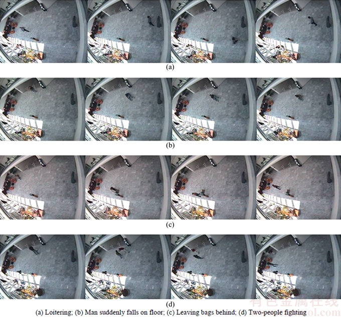
Fig. 1 CAVIAR dataset:
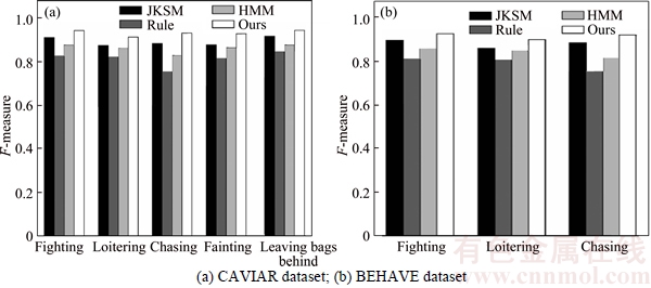
Fig. 2 Comparison of related algorithms:
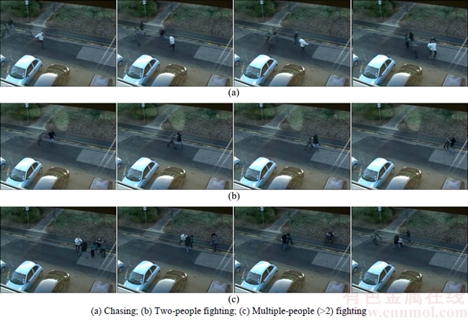
Fig. 3 BEHAVE dataset:
6 Conclusions
1) A new approach for abnormal behavior detection based on causality analysis is proposed. This method can be used for both single and multiple object anomalies detection.
2) New behavior features is introduced. The low level visual features, including trajectory shape descriptor, speeded up robust features and histograms of optical flow, are used to describe individual behavior on the structural and motioning side. And causality features are introduced to depict the interaction information among a set of objects. Finally, the bag of words method is used to merge two types features together.
3) The sparse representation is applied to anomaly detection. The proposed method could cope with feature noisy and uncertainty.
4) Two databases were used to test the proposed methods: the CAVIAR datasets and the BEHAVE dataset. The experimental results show that the proposed method is applicable in different databases and has a higher recognition validity than the other state-of-the-art methods.
References
[1] CUI X, LIU Q, GAO M, METAXAS D N. Abnormal detection using interaction energy potentials [C]// IEEE Computer Vision and Pattern Recognition. Colorado Springs: IEEE, 2011: 3161�C3167.
[2] PICIARELLI C, FORESTI G L. Trajectory-based anomalous event detection [J]. IEEE Transactions on Circuits and Systems for Video Technology, 2008, 18(11): 1544�C1554.
[3] DEEPIKA R, PRASATH V S A, INDHUMATHI M, KUMAR P M A, VAIDEHI V. Anomalous event detection in traffic video surveillance based on temporal pattern analysis [J]. Journal of computers, 2017, 12(2): 190�C199.
[4] KWAK S, BYUN H. Detection of dominant flow and abnormal events in surveillance video [J]. Optical Engineering, 2011, http://dx.doi.org/10.1117/1.3542038.
[5] MAHADEVAN V, LI W, BHALODIA V, VASCONCELOS N. Anomaly detection in crowded scenes [C]// IEEE Computer Vision and Pattern Recognition. San Francisco: IEEE, 2010: 1975�C1981.
[6] WU S, MOORE B E, SHAH M. Chaotic invariants of Lagrangian particle trajectories for anomaly detection in crowded scenes [C]// IEEE Computer Vision and Pattern Recognition. San Francisco: IEEE, 2010: 2054�C2060.
[7] KRATZ L, NISHINO K. Anomaly detection in extremely crowded scenes using spatio-temporal motion pattern model [C]// IEEE Computer Vision and Pattern Recognition. Miami Beach: IEEE, 2009: 1446�C1453.
[8] MEHRAN R, OYAMA A, SHAH M. Abnormal crowd behavior detection using social force model [C]// IEEE Computer Vision and Pattern Recognition. Miami Beach: IEEE, 2009: 935�C942.
[9] BENEZETH Y, JODIN P, SALIGRAMA V, ROSENBERGER C. Abnormal events detection based on spatio-temporal co-occurences [C]// IEEE Computer Vision and Pattern Recognition. Miami Beach: IEEE, 2009: 2458�C2465.
[10] CONG Y, YUAN J S, LIU J. Sparse reconstruction cost for abnormal event detection [C]// IEEE Computer Vision and Pattern Recognition. Colorado Springs: IEEE, 2011: 3449�C3456.
[11] KIM J, GRAUMAN K. Observe locally, infer globally: A space-time MRF for detecting abnormal activities with incremental updates [C]// IEEE Computer Vision and Pattern Recognition. Miami Beach: IEEE, 2009: 2913�C2920.
[12] SALIGRAMA V, CHEN Z. Video anomaly detection based on local statistical aggregates [C]// IEEE Computer Vision and Pattern Recognition.Providence: IEEE, 2012: 2112�C2119.
[13] REDDY V, SANDERSON C, LOVELL B C. Improved anomaly detection in crowded scenes via cell-based analysis of foreground speed, size and texture [C]// IEEE Computer Vision and Pattern Recognition. Colorado Springs: IEEE, 2011: 55�C61.
[14] NALLAIVAROTHAYAN H, FOOKES C, DENMAN S. An MRF based abnormal event detection approach using motion and appearance features [C]// IEEE International Conference on Advanced Video and Signal based Surveillance. Seoul: IEEE, 2014: 343�C348.
[15] FU Z Y, HU W M, TAN T I. Similarity based vehicle trajectory clustering and anomaly detection [C]// IEEE International Conference on Image Processing. Genoa: IEEE, 2005: 2029�C2032.
[16] HU W M, XIAO X, FU Z Y. A system for learning statistical motion patterns [J]. IEEE Transactions on Pattern Analysis & Machine Intelligence, 2010, 28(9): 1450�C1464.
[17] BERA A T, KIM S, MANOCHA D. Realtime anomaly detection using trajectory-level crowd behavior learning [C]// IEEE Conference on Computer Vision and Pattern Recognition. Las Vegas: IEEE, 2016: 50�C57.
[18] JEONG H, CHANG H J, JIN Y C. Modeling of moving object trajectory by spatio-temporal learning for abnormal behavior detection [C]// IEEE International Conference on Advanced Video and Signal-Based Surveillance. Klagenfurt: IEEE, 2011: 119�C123.
[19] YANG W Q, GAO Y, CAO L B. TRASMIL: A local anomaly detection framework based on trajectory segmentation and multi-instance learning [J]. Computer Vision and Image Understanding, 2013, 117(10): 1273�C1286.
[20] LI C, HAN Z, YE Q, JIAO J. Visual abnormal behavior detection based on trajectory sparse reconstruction analysis [J]. Neurocomputing, 2013, 119(7): 94�C100.
[21] ZHAO B, LI F F, XING E. Online detection of unusual events in videos via dynamic sparse coding [C]// IEEE Conference on Computer Vision and Pattern Recognition. Colorado Springs: IEEE, 2011: 3313�C3320.
[22] REN H M, LIU W F, ESCALERA S, MOESLUND T B. Un- supervised behavior-specific dictionary learning for abnormal event detection [C]// The British Machine Vision Conference. Swansea Bay: Springer, 2015: 135�C144.
[23] WANG X, MA X, GRIMSON W. Unsupervised activity perception in crowded and complicated scenes using hierarchical Bayesian models [J]. IEEE Transactions on Pattern Analysis and Machine Intelligence, 2009, 31(3): 539�C555.
[24] VASWANI N, ROY-CHOWDHURY A, CHELLAPPA R. Shape activity: A continuous state hmm for moving/deforming shapes with application to abnormal activity detection [J]. IEEE Transactions on Image Processing, 2005, 14(10): 1603�C1616.
[25] MO X, MONGA V, BALA R, FAN Z G. Adaptive sparse representations for video anomaly detection [J]. IEEE Transactions on Circuits and Systems for Video Technology, 2014, 24(4): 631�C645.
[26] HAN M, XU W, TAO H. An algorithm for multiple object trajectory tracking [C]// IEEE Conference on Computer Vision and Pattern Recognition. Washington: IEEE, 2004: 864�C871.
[27] CUI X Y, LIU Q S, GAO M C, METAXAS D N. Abnormal detection using interaction energy potentials [C]// IEEE Conference on Computer Vision and Pattern Recognition. Colorado Springs: IEEE, 2011: 3161�C3167.
[28] XIA L M, YANG B J, TU H B. Recognition of suspicious behavior using case-based reasoning [J]. Journal of Central South University, 2015, 22(1): 241�C250.
[29] GRANGER C. Investigating causal relations by econometric models and cross-spectral methods [J]. Econometrica, 1969, 37(3): 424�C438.
[30] XIA L M, HAN F, WANG J. Complex human activities recognition using interval temporal syntactic model [J]. Journal of Central South University, 2016, 23(10): 2578�C2586.
[31] SHI J, TOMASI C. Good features to track [C]// IEEE Conference on Computer Vision and Pattern Recognition. Seattle: IEEE, 1994: 593�C600.
[32] LAPTEV I. On space-time interest points [J]. International Journal of Computer Vision, 2005, 1(2, 3): 432�C439.
[33] ZHOU Y, YAN S, HUANG T. Pair-activity classification by bi- trajectory analysis [C]// IEEE Conference on Computer Vision and Pattern Recognition,Anchorage, AK, IEEE, 2008: 3682�C3689.
[34] NI B P, YAN SC, KASSIM A. Recognizing human group activitieswithlocalizedcausalities [C]//IEEE Conference on Computer Vision and Pattern Recognition, Miami Beach: IEEE, 2009: 1470�C1477.
[35] NESTEROV Y. Gradient methods for minimizing composite objective function [J]. Mathematical Programming, 2013, 140(1): 125�C161.
(Edited by FANG Jing-hua)
Cite this article as:
WANG Jun, XIA Li-min. Abnormal behavior detection by causality analysis and sparse reconstruction [J]. Journal of Central South University, 2017, 24(12): 2842�C2852.
DOI:https://dx.doi.org/https://doi.org/10.1007/s11771-017-3699-yFoundation item: Project(50808025) supported by the National Natural Science Foundation of China; Project(20090162110057) supported by the Doctoral Fund of Ministry of Education, China
Received date: 2016-12-29; Accepted date: 2017-03-15
Corresponding author: XIA Li-min, Professor, PhD; Tel: +86�C13974961656; E-mail: xlm@mail.csu.edu.cn
Abstract: A new approach for abnormal behavior detection was proposed using causality analysis and sparse reconstruction. To effectively represent multiple-object behavior, low level visual features and causality features were adopted. The low level visual features, which included trajectory shape descriptor, speeded up robust features and histograms of optical flow, were used to describe properties of individual behavior, and causality features obtained by causality analysis were introduced to depict the interaction information among a set of objects. In order to cope with feature noisy and uncertainty, a method for multiple-object anomaly detection was presented via a sparse reconstruction. The abnormality of the testing sample was decided by the sparse reconstruction cost from an atomically learned dictionary. Experiment results show the effectiveness of the proposed method in comparison with other state-of-the-art methods on the public databases for abnormal behavior detection.
