Improved differential evolution algorithm for solving constrained problem

ZHAO Juan(赵娟)^{1, 2}, CAI Tao(蔡涛)^{1, 2}, DENG Fang(邓方)^{1, 2}, SONG Xiao-qing(宋晓青)¹

(1. School of Automation, Beijing Institute of Technology, Beijing 100081, China;

2. Beijing Key Laboratory of Automatic Control System, Beijing Institute of Technology, Beijing 100081, China)

Abstract: In order to solve sequence constrained optimization problems, a differential evolution algorithm with mapping (MDE) is presented. By mapping the sorting variables to random coefficient range [0,1], the constrained problems can be turned into unconstrained. In addition, differential evolution algorithm (DE) with self-adapting parameters is applied to accelerate the convergence rate. The results show the high efficiency of the method to solve such constrained problems.

Key words: DE algorithm; sequence constrained problem; self-adapting parameter; mapping

CLC number:TP391                  Document code: A             Article ID: 1672-7207(2011)S1-0154-05

1 Introduction

Differential evolution (DE) algorithm based on genetic algorithm (GA) and other evolutionary algorithms (EA) was presented by Storn et al^[1-2]. DE is a parallel searching algorithm which applies real vector coding to search randomly in continuous space. Moreover, DE, by minimizing nonlinear, non- differentiable, continuous space function, has good global convergence and robustness, and is suitable to solve numerical optimization problems. In the first international IEEE contest on evolutionary optimization held in 1995, DE is proven to converge the fastest among various EA algorithms verified on site. Compared with other evolutionary algorithms, DE has advantages of easiness in concept, few control parameters, fast convergence, no need of initial value and derivation computation, so it is applied to many fields^[3-4]. Currently, there are many methods to improve DE. Some of them are modified in convergence speed and global optimization. A differential evolution algorithm called AdaptDE is presented in Ref. [5], in which self-adaptive mechanisms are applied to control parameters. Therefore, the optimal control parameters for different optimization problems can be obtained without user interaction. An improved self-adaptive differential evolution algorithm (IADE) with parameters self-adaptive and a new mutation strategy is given in Ref. [6]. Ref. [7] proposes a new DE algorithm with a second enhanced mutation operator. To improve exploration ability, a new framework with a single population is adopted, and a second enhanced mutation operator is used to ensure the exploitation of the previous knowledge about the fitness landscape. In Ref. [8], double mutation operation and chaos differential evolution are presented to improve DE algorithm’s optimization performance. Others are mentioned for solving constrained optimization problems. Ref. [9] proposes a constrained self-adaptive differential evolution algorithm. This algorithm is an enhancement of a previous work that requires no parameter settings at all. In Ref. [10], a modified Differential Evolution with hybrid mutation and new selection rules is proposed to solve the hard constrained optimization problem.

Due to the independence of the variables, DE algorithm can directly solve most optimization problems. However, for other optimization problems, especial impulsive control problem, aforementioned algorithms no longer work. Because there is order between variables, that is, the latter variable relies on the former one. So a novel DE algorithm with mapping (MDE) is proposed in this paper to solve problems with constrained variables, in which ordered vectors are mapped to random coefficient ranged from 0 to 1. By solving the random coefficients, we can get the original ordered vectors indirectly. Experimental results show that the algorithm is very effective to solve such sorting problems.

2 Constrained optimization problem

Suppose a simplified model:

s.t.  x_min≤x₁≤x₂≤…≤x_n≤x_max

x_j-x_i≥?x, for j≥i            (1)

The model is a constrained sorting problem, and DE algorithm can not be used to solve directly. Therefore it’s necessary to improve the algorithm. DE algorithm initializes population randomly in D dimensional bounded space, and it can not guarantee the order of target vector. The sorting method can be applied to solve numerical sorting problem from small to big. But if we sort the vector after algorithm initialization, during the mutation operation, the order sequences can be destroyed easily. Ref. [11] presents a method based on the values of individuals themselves, thus the sorted population is (x₁, x₂, …, x_NP), x_i≤x_j, if i＜j, and i, j∈[1, N_P]. In Ref. [12], an approach based on the fitness valves is proposed, the sorted population is (x₁, x₂, …, x_NP), f(x_i)≤f(x_j), if   i＜j, and i, j∈[1, N_P]. In this paper, the sequence is arranged according to the values of variables of each individual, variables would be arrayed as follows:

(x_i1, x_i2, …, x_iD), x_ik≤x_ij, if k＜j, k, j∈[1, D], i∈[1, N_P].

3 DE algorithm

3.1 Basic DE algorithm

DE is an optimization algorithm based on the theory of swarm intelligence, which the optimization search is guided by cooperation and competition among individuals within populations. Compared to GA algorithm, DE reserves the population-based global search strategy, using real coding, reducing the complexity of genetic operation. DE has the same evolutionary processes with GA algorithms: mutation, crossover and selection.

3.1.1 Initialization

DE takes N_P real parameter vectors with D dimension as the population of every generation; each individual is expressed as (i=1, 2, …, N_P), where i is the sequence of the individual in the population; N_P is population size which is constant in the process of minimization. Suppose the boundary of the parameter variables is , then

i=1, 2, …, N_P; j=1, 2, …, D        (2)

where rand[0,1] is a random value homogeneous distributed in area (0, 1).

3.1.2 Mutation

For each target vector x_i,G, i=1, 2, …, N_P, a new temporary individual is generated:

        (3)

where randomly selected r₁, r₂ and r₃ are different from each other, and are also different from the number of target vector i, so it must satisfy with N_P≥4. Scale factor F is a real constant factor with the value in [0.5, 1], usually.

3.1.3 Crossover

In order to increase the diversity of parameter vector interference, introduce crossover operation. The test vector becomes

i=1, 2, …, N_P; j=1, 2, …, D       (4)

where randb(j)∈[0,1] is a random number generated for each dimension j and rnbr(i)∈(1, 2, …, D) is a random integer generated for each trial vector which ensures that u_i,G+1 takes at least one parameter from v_i,G+1. C_R∈[0,1] is the crossover probability.

3.1.4 Selection

In order to determine whether the vector u_i,G+1 becomes an individual of the next generation population, DE compares the test vector u_i,G+1 with the target vector of current operation x_i,G according to greedy criterion. If the fitness of the former is better than the latter, x_i,G is replaced by u_{i,G+1 in G+1 generation, otherwise xi,G} would be reserved.

         (5)

3.1.5 Boundary conditions

The target vector is constrained by boundary conditions, so it’s necessary to ensure that the new individual parameter values in the feasible region. In this paper, new individuals that do not meet boundary conditions would be replaced by the vector randomly generated in the feasible region. If ＜ or ＞, then

i=1, 2, …, N_P; j=1, 2, …, D        (6)

3.2 DE algorithm with mapping

DE algorithm searches optimal solution in a bounded space, so the limit for each variable must be determined. In this paper, the target vector  is constrained by  , for j＞i, so the limit of each variable x_i is no longer in [x_min, x_max], and needs to be redefined.

The low limit of solution space for variable x₁ is given as x_min, and to ensure that the last variable x_n≤x_max, the up limit of the solution space should be , then the solution space of the second variable x₂ becomes  with the up limit . And so on, the up and low limit of solution space for each variable will be determined.

            (7)

x_i can be expressed as follows:

        (8)

where r₁, r₂,…, r_n range [0, 1]. The target vector {x₁, x₂, …, x_n} changes into {r₁, r₂, …, r_n}, and {x₁, x₂, …, x_n} can be optimized by optimizing {r₁, r₂, …, r_n} indirectly.

  From this method, the target vector becomes {r₁, r₂, …, r_n}, and r_i is independent of each other. So DE can be adopted to solve. First obtain the optimal solution of {r₁, r₂, …, r_n}, and then get {x₁, x₂, …, x_n} from  Eqs.(7) and (8), with which the fitness can be calculated. By mapping the sorting variables to random coefficient range [0,1], the constrained problems can be turned into unconstrained. And the solution space is also reduced to [0,1], which improves the search efficiency of the algorithm.

3.3 DE algorithm parameters setting

DE has three control parameters, i.e., population size N_P, mutation factor F and crossover operator C_R. N_P is generally between 5D and 10D (D is the number of variables in target vector), and is not less than 4, otherwise it is impossible to mutation. The value of N_P has an influence on the diversity of group directly. A larger N_P leads to a more complicated group and higher opportunity to obtain the optimal solution, meanwhile, a higher computational cost.

Mutation factor F determines the diversity and converge speed of the group. A small value of F will speed up the convergence while a large one slows it down. However, a too small value of F may result in non-optimal solution early while a large one can avoid this situation^[13]. Value of C_R will influence the degree of individual participation. A large C_R can enhance the local exploration ability, while a small C_R is conductive to maintain the diversity of group, but hinders the generation of new individuals^[14].

Self-adapting parameters adjustments according to fitness are applied to obtain high convergence speed and global optimization. In this paper, C_R is set according to the formula in Ref. [14]. To those individuals with poor fitness, larger C_R is taken to make the mutation individuals have a large contribution to trail ones, causing them to be eliminated faster. While to those individuals with better fitness, smaller C_R is taken to make the individual have greater opportunity to evolve into the new population. F is setting according to the formula in Ref. [13]. It will be given a small value when the individual has good fitness, so that the algorithm will search in local areas, and have higher opportunity to access improved solutions. When the individual has bad fitness, a large value will be taken to maintain the diversity of the group. Self-adapting parameters are set by follows:

     (9)

where C_Ri is the value of C_R of current ith individual, and f_i is the fitness of it, f_max and f_min are the best and worst fitness of current population.

          (10)

where i is the arrangement location after the population is descending sorted, F_max and F_min are the maximum and minimum value of scale factor, and 0≤F_min≤F_max≤2.

Setting F and C_R with this method, the algorithm can have strong global search ability in initial stage of evaluation to find the feasible global optimum. Meanwhile, it has strong local search ability in the latter stage, which improves the DE convergence speed and solution precision.

3.4 Algorithm process

Step 1: Decide the DE control parameters and search space of target vector. DE control parameters include population size, mutation operator, crossover operator, the maximum evolution generation, termination conditions, etc.

Step 2: Initialize population randomly, and set evolution generation k = l.

Step 3: Evaluate the initial population, i.e. calculate fitness of each individual of initial population.

Step 4: Decide whether end condition or maximum evolutionary generation is met. If so, stop evolution and the best individual at this time will be output as the solution; if not, continue.

Step 5: Mutation and crossover. Check boundary conditions, and then get a temporary population.

Step 6: Evaluate the temporary population, and calculate the fitness of each individual of it.

Step 7: Select operation, get a new population.

Step 8: Set evolution generation k=k+1, and go to step 4^[15].

4 Numerical example

Example 1：Sparse circular arrays^[16]: Consider a circular array with radius  (m is a constant,  is wavelength), which is composed of N antenna elements with different distances, d_i is azimuth of the ith element, the direction of beam is , then the pattern function can be expressed as:

   (11)

where A_i is the magnitude of ith (i≤N) element,  is the azimuth pointing to x-axis positive direction, and  is the pitch angle pointing to z-axis positive direction. When , the array pattern function becomes:

     (12)

The pattern maximum relative sidelobe level M_SLL is:

   (13)

where S is sidelobe area of pattern, if the zero power point of main lobe is , then   and ≤≤360°}. Make the first unit’s azimuth 0°, and two adjacent units’ azimuth interval meet the range , 1≤j＜i≤N, d_c is constant, so the optimal modal is: , where

The following data are given: d_c=14.364 1, A_i=4d_c (i=1, 2, …, N), , N=16, R=2λ.

The parameters of the adopted DE are: C_Rmin=0.2, C_Rmax=0.9, F_min=0.4, F_max=0.9, N_P=100, D=16, G=200.

The test independently runs 10 times, and the best solutions are shown in Fig.1. The best fitness is min(J(d))=-12.506 1, which is approximate to or even better than the known result in Ref. [16]. The case shows global convergence of the algorithm.

Example 2：Impulsive control model of Antiaircraft Guided Munitions^[17] is shown in Fig.1.

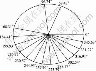
Fig.1 Simulation result

The state equations are:

      (14)

where S is the reference area of the projectile, m denotes the mass, g is the gravitational constant, c_x is the resistance coefficient, q is the function of velocity v, q=1/(2ρv²), and ρ is air density.

,

              (15)

Optimization model is:

s.t.

t_min≤t₁＜t₂＜…＜t_n≤t_max

t_i-t_i-1≥?t (i=2, 3, …, n)        (16)

where x_f, y _f, z_f are the values of x, y, z when t=t_f. The following data are given: n=8, m=2.8, g=9.8, P=500, t₀=0, t_f=10, x₀=0, y₀=0, z₀=0, v₀=960, θ₀=1.13, ψ₀=0, x_f=2 274, y_f=4 627.1, z_f=-36.2.

The parameters of the adopted DE are: C_Rmin=0.2 m, C_Rmax=0.9, F_min=0.5, F_max=0.9, N_P=80, D=16, G=300.

The test independently runs 5 times, and all simulation results satisfy the requirements. The best solution is (1.73, 2.32, 1.595 8, 2.23, 2.79, 1.88, 2.04, 1.79, 5.22, 5.25, 5.28, 5.33, 5.35, 5.45, 5.47, 5.50), which is shown in Fig.2, and Min J=5.61. The case certifies that the improved algorithm is effective to solve this impulsive control problem.

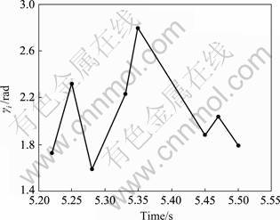
Fig.2 Simulation result

5 Conclusions

An improved DE algorithm is proposed to solve optimization problems with sequence constraint. Constrained problems can be reduced into unconstrained ones by adopting DE algorithm with mapping, which also narrows the search space of variables greatly, and improves the efficiency of algorithm. An adaptive method is also used to set the value of C_R and F of DE, which improves the convergence speed. Finally, two examples are cited to demonstrate the validity of the method. Results show the high global searching capability and fast convergence speed of the algorithm to solve such constrained optimization problems.

References

[1] Storn R, Price K. Differential evolution—A simple and efficient adaptive scheme for global optimization over continuous spaces[R]. California: International Computer Science Institute, 1995: 22-25.

[2] Storn R, Price K. Differential evolution-A simple and efficient heuristic for global optimization over continuous spaces[J]. Journal of Global Optimization, 1997, 11(4): 341-359.

[3] Yungchien L, Kaoshing H, Fengsheng W. Co-evolutionary hybrid differential evolution for mixed-integer optimization problems[J]. Engineering Optimization, 2001, 33(6): 663-682.

[4] Shih-Lian C, Chyi H. Optimal approximation of linear systems by a differential evolution algorithm[J]. IEEE Transactions on Systems, Man and Cybernetics: A, 2001, 31(6): 698-707.

[5] Wu Z, Houkuan H, Bei Y, et al. A modified differential evolution algorithm with self-adaptive control parameters[C]//ISKE 2008. The 3rd International Conference. Xiamen, China, 2008: 524-527.

[6] Wenjing J, Liqun G, Yanfeng G, et al. An improved self-adapting differential evolution algorithm[C]//Computer Design and Applications (ICCDA). Qinghuangdao, China, 2010: 341-344.

[7] Changshou D, Bingyan Z, Anyuan D, et al. New differential evolution algorithm with a second enhanced mutation operator[C]//Intelligent Systems and Applications. Hubei, China, 2009: 1-4.

[8] Jin H, Liu M. An improved differential evolution algorithm for optimization[C]//Control, Automation and Systems Engineering, 2009 (CASE 2009). IITA International Conference. Zhangjiajie, China, 2009: 659-662.

[9] Worasucheep C. Solving constrained optimization problems with a self-adaptive differential evolution algorithm[C]//Electrical Engineering/Electronics, Computer, Telecommunications and Information Technology. Pattaya, Chonburi, 2009: 686-689.

[10] Changshou D, Bingyan Z, Anyuan D, et al. Modified differential evolution for hard constrained optimization[C]//Computational Intelligence and Software Engineering. Wuhan, China, 2009: 1-4.

[11] Tassing R, Wang D, et al. Gene sorting in differential evolution[C]// The 6th International Symposium on Neural Networks, ISNN 2009. 2009: 663-674.

[12] Lou Y, Li J L, Wang Y S. A differential evolution algorithm based on ordering of individuals[C]//Industrial Mechatronics and Automation (ICIMA) 2010 2nd International Conference. Wuhan, China, 2010: 105-108.

[13] Dalin R, Guobiao C. Improved differential evolution algorithm for fast simulation and its application[J]. Journal of Astronautics, 2010, 31(3): 793-797. (in Chinese)

[14] XU Jing-ting. The research and applications of modified differential evolution algorithm[J]. Electronics R & D, 2010(5): 10-13. (in Chinese)

[15] Wan D. Differential evolution algorithm and its application[J]. Science Technology and Engineering, 2009, 9(22): 6673-6676. (in Chinese)

[16] Ziyang B, Kesong C. Sparse circular arrays method based on modified DE algorithm[J]. Systems Engineering and Electronics, 2009(3): 497-499. (in Chinese)

[17] YANG Hong-wei, DOU Li-hua, GAN Ming-gang. A particle swarm optimization for fuel-optimal impulsive control problems of guided projectile[C]//Control and Decision Conference (CCDC). Beijing: China, 2010: 3034-3038.

(Edited by CHEN Can-hua)

Received date: 2011-04-15; Accepted date: 2011-06-15

Foundation item: Project (60925011) supported by the National Science Fund for Outstanding Youths

Corresponding author: ZHAO Juan(1986-), Master, Major in Control System Simulation; Tel: +86-13401099660; E-mail: juantime@163.com