

J. Cent. South Univ. (2020) 27: 1917-1938
DOI: https://doi.org/10.1007/s11771-020-4420-0

Automated extraction of expressway road surface from mobile laser scanning data
TRAN Thanh Ha, TAWEEP Chaisomphob
School of Civil Engineering and Technology, Sirindhorn International Institute of Technology, Thammasat University, Pathumthani 12121, Thailand
 Central South University Press and Springer-Verlag GmbH Germany,part of Springer Nature 2020
Abstract:
This paper presents a voxel-based region growing method for automatic road surface extraction from mobile laser scanning point clouds in an expressway environment. The proposed method has three major steps: constructing a voxel model; extracting the road surface points by employing the voxel-based segmentation algorithm; refining the road boundary using the curb-based segmentation algorithm. To evaluate the accuracy of the proposed method, the two-point cloud datasets of two typical test sites in an expressway environment consisting of flat and bumpy surfaces with a high slope were used. The proposed algorithm extracted the road surface successfully with high accuracy. There was an average recall of 99.5%, the precision was 96.3%, and the F1 score was 97.9%. From the extracted road surface, a framework for the estimation of road roughness was proposed. Good agreement was achieved when comparing the results of the road roughness map with the visual image, indicating the feasibility and effectiveness of the proposed framework.
Key words:
mobile laser scanning; segmentation; road surface; expressway; voxelization; point cloud��
Cite this article as: TRAN Thanh Ha, TAWEEP Chaisomphob. Automated extraction of expressway road surface from
mobile laser scanning data [J]. Journal of Central South University, 2020, 27(7): 1917-1938. DOI: https://doi.org/10.1007/s11771-020-4420-0.
1 Introduction
A road network is used for the daily activities of citizens including transport services, goods, and people [1]. A proper design with high quality and management (with maintenance) of the road network system is important for linking an urban region to a rural region, a city to another city, or a country to its neighbors. A good design can also reduce the time and cost of transportation. Expressway/highway systems are an integral part of a road network, which is designed to handle traffic congestion, snarl-ups, and traffic collisions inside a city and also reduce the travel time from city to city.
Low quality of expressway surfaces can lead to severe traffic casualties [2]. Periodic maintenance and assessment of the surfaces should, therefore, be checked regularly by the maintenance expressway authorities to ensure the convenience, comfort, and safety of drivers. Conventionally, all expressway information data were manually collected by on-site inspectors. This information was then converted to a digital version when updating the management system of an expressway. The collected expressway information data consisted of expressway facilities (including lighting poles, noise barriers, traffic signs, overhead signs, telecommunication stations, emergency phones, and traffic safety equipment) and expressway surface features (including maintenance holes, road slope, lane width, lane number, road markings, road curbs, and road crack status). However, due to the complex and large scale of an expressway, the traditional method (e.g., total station or real-time kinematic surveying combined with image capture) had disadvantages such as being tedious, time-consuming, expensive, and possibly obstructive to the normal traffic flow [3].
Recently, remote sensing in the form of aerial and satellite images and laser scanning has emerged, allowing the capture of three-dimensional (3D) topographic data for a road network, accurately and quickly [4-6]. Laser scanning integrated into a vehicle, called mobile laser scanning (MLS) can capture 3D information of road surfaces and their surrounding objects. MLS can produce highly dense data (8000 points/m2) with an absolute accuracy of about 5 mm [7]. There are wide applications of MLS data in road engineering, which can include 3D geometric road reconstruction [8], road surface damage identification [9], and extraction of road markings and traffic signs [10-12].
For most applications of MLS data, a point cloud of a road surface needs to be extracted. However, a big challenge is to deal with the massive volume of point clouds since MLS can acquire up to 2000000 points/s and 62 GB of data per km of road [13]. This paper proposes an efficient and robust approach to automatically extract road surfaces from MLS point clouds. The approach is a combination of the voxel model and the region growing segmentation method, to accelerate the road surface extraction. Subsequently, the road surface quality is reported based on the point cloud of the extracted road surface, which allows infrastructure authorities to identify any anomaly of the road surface.
The rest of the paper is organized as follows. Past studies are reviewed in Section 2. In Section 3, a voxel-based method is presented, and the framework for the estimation of road roughness based on the extracted road surface is also introduced. Two test sites are used to demonstrate the proposed method in Section 4. Section 5 concludes this study.
2 Related work
To date, many remote sensing technologies have been widely used to extract geometric and semantic information from road networks including road surfaces and edges [6, 14-18], road cross-sections [19, 20], road markings [10, 11, 21], and road furniture [12, 22, 23]. Those remote sensing resources can be satellite and aerial images, and laser scanning. This survey is focused on using laser scanning data, particularly mobile laser scanning (MLS), for road extraction, while others are presented elsewhere [4, 24-26]. State-of-the-art road extraction can be roughly classified into two groups: (1) road edge and (2) road surface.
In the former category, algorithms were used to detect the road edge first, and then the data points of the road surface were extracted in such a way that all points were located inside the road edges [1, 27-32]. MCELHINNEY et al [27] divided point clouds into a set of cross-sections. The points in each cross-section were fitted by a 2D cubic spline. Then, the slope of the spline was computed. From the calculated slope, the candidate road-edge points were selected based on the peaks and troughs of the slope. To correctly filter the road-edge points from the candidate road-edge points, additional information of the data points such as echo width and intensity was required. ZHANG [28] proposed a method to recognize the road edge and road surface based on a combination of elevation information and prior knowledge of the minimal road width. IBRAHIM et al [29] extracted the road curb based on 3D density-based segmentation. A drawback of their method is the difficulty in detecting the curb at the road intersection due to the sensitivity of the parameter thresholds and the noise data. Moreover, additional information such as the predefined value of road width was required for setting some thresholds. YANG et al [30] generated the road curbs, which were then used to reconstruct the road surface, using curb-based and scan line-based approaches. This method may face some difficulty when the MLS point clouds were not ordered data or collected from a 2-laser scanner. Moreover, their proposed method was time- consuming since it required the complex geometry of all points in the curb point extraction step. GUAN et al [1] developed the slope-based and elevation-based method to extract the road curbs and road surface. Using sparse curb points (i.e., two points only) in each cross-section profile to form road edges, the edge of the road with a large curvature change cannot be well determined. To overcome this limitation, WANG et al [31] introduced a local normal saliency-based approach for extracting the road curb. By partitioning the road into overlapping road segments, the dense curb points in each road segment were extracted (instead of only two curb points in each cross-section profile, as in the previous method). Nevertheless, their method may fail for extracting road curb points at a T-intersection due to the impact of curved trajectory data. CABO et al [32] applied the line cloud concept for automatically extracting an asphalt road. However, to generate line clouds from 3D data point, their method required the structured input point cloud data in such a way that the points were sorted by their timestamps.
Apart from using the road edge as the preparatory step for extracting the road surface, several methods were used to extract the 3D point cloud of a road surface with additional road feature information, based on some assumptions of the road surface. MIYAZAKI et al [33] employed a line-based region-growing approach which was used to create the road surface with an assumption that most of the artificial road surface was planar. Their method was limited by unstructured input data (i.e., the data did not consist of scan line information and navigation). WU et al [34] developed an adaptive alpha shapes algorithm to detect the ground surface in an urban environment. YANG et al [15] developed the binary kernel descriptor that represented 3D local features, to extract the road curbs and road surfaces. However, the method was expensive (computation) due to the kernel density estimation step. YADAV et al [3] performed the road surface extraction using a density- and intensity-based approaches. Some additional road information, such as roughness of the road, road spatial geometry, intensity, and density of point cloud data, was required. BALADO et al [6] proposed a method to extract and classify the urban ground component (e.g., road surfaces, curbs, stairs, ramps, and sidewalks) from MLS point cloud data based on a combination of topological and geometrical information. However, their method was limited by the irregular topography of the road surface such as bumpy or uneven roads.
In summary, many methods were proposed to develop an algorithm for automatic extraction of the road surface by using the 3D point cloud data with structured or unstructured pattern data. However, these approaches usually required additional information such as roughness of the road, road spatial geometry, point density variation [3, 29, 30], echo width [27], returned intensity [3, 15], GPS time [30, 32], ordered data [30, 32, 33], road width [27-29], smooth road surface [6, 28, 33], or distance to the trajectory [27, 31]. It is worth noting that our expressway had significant elevation variation in the vertical cross-section profile along the road. Thus, the reviewed methods may not be relevant. To overcome these disadvantages, a method that integrates the region growing segmentation method and the voxel model is proposed to enhance the robustness and efficiency of the expressway road surface extraction.
3 Proposed method
A goal of the paper is to propose an efficient, robust method for processing a massive amount of MLS data for extracting the road surface of an expressway. The proposed method for road surface extraction consists of three main steps (Figure 1): 1) construct a voxel model for point cloud data; 2) extract the road surface based on voxel-based region growing; and (3) refine the road surface extraction in Step 2 by considering the similarity of local surfaces. First, the octree representation was employed to subdivide a 3D space into small voxels. Subsequently, voxel-based region growing was used to extract the points of the road surface. Finally, the unallocated points that are missing in the region growing segmentation step were recovered in the refinement process.
When collecting data from MLS, noise and outliers inevitably exist in point cloud due to reflection of the different object surface and sensor imperfections. These outlier points may lead to a wrong estimation of the local road surface��s feature in the following algorithm; thus, a preprocessing step is necessary to remove these points, which was implemented by a statistical outlier removal approach [35]. For each point �� in raw 3D point cloud, the average distance  from �� to its k-neighbor points was computed (di is the distance from the point �� to the i-th neighbor point). Then, the mean �� and standard deviation �� of the distance
 were calculated. The points were considered as outliers if the average distance to its k-neighbors satisfied>(��+��). In this research, noise removal was semi-automatic done by using an open-source software CloudCompare V2.10 [36].
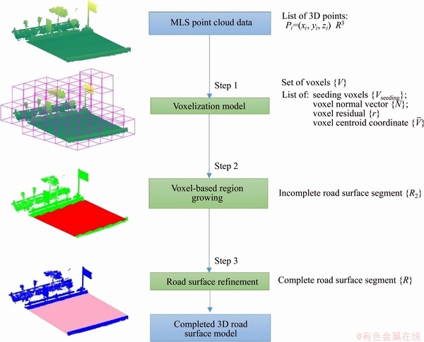
Figure 1 Workflow for road surface extraction from MLS point cloud data
After eliminating the noise points, many points of moving objects are still present in point clouds. These irrelevant points significantly influence a voxel-based region growing algorithm. Therefore, the moving objects should be eliminated from point clouds, which was implemented by using CloudCompare software.
3.1 Road surface extraction
3.1.1 Voxelization
In the first step, from the set of 3D point cloud data Pi=(xi, yi, zi) R3, i=1, ��, n, where n is the number of data points, an octree representation was employed to recursively subdivide an initial bounding box into smaller cubes (also called voxels) until a termination condition is reached (Figure 2). The initial bounding box enclosing the entire input data can be defined as the origin O (xmin, ymin, zmin) and the length in x, y and z directions, which are computed as in Eq. (1):
��x=��y=��z=max[|xmax-xmin|, |ymax-ymin|,|zmax-zmin|] (1)
where (xmin, ymin, zmin) and (xmax, ymax, zmax) are the minimum and maximum of the x, y, z coordinates of the point cloud, respectively.
In octree subdivision, several terminations have been proposed, for example, the minimum voxel size [37], the minimum number of points within the voxel [38], or the highest depth of the tree [39]. The voxel size was chosen as the termination condition in this study. For each voxel, a pair of coordinates (A and B) was used to store the top left and bottom right of the voxel to describe the voxel geometry. Moreover, if the voxel contains no less than 3 data points, the voxel was considered to be ��full��; otherwise, the voxel was classified as ��empty��. It is noted that the subdivision was applied to only the full voxels. Finally, a set of full voxels V on leaf nodes was used as the input data for a voxel-based region-growing algorithm.
Next, to extract a point cloud of a road surface by voxel-based region-growing segmentation, features of each full voxel were computed, which were a normal vector and residual. Since the road surface was an objective of this segmentation and voxels were assumed to describe a patch of the road surface, the points within the voxels should represent a planar surface. Principal component analysis (PCA) [40] was employed to estimate the normal vector of each full voxel. The normal vector was the eigenvector corresponding to the smallest eigenvalue determined from covariance matrix CV (Eq. (2)). Moreover, the residual was defined as the root mean square of the perpendicular distances from the points to the fitting surface, which is expressed in Eq. (3).
 (2)
(2)
where is the center of the point pi=(xi, yi, zi) within full voxel, which is also considered the voxel centroid, and m is the total number of pi.
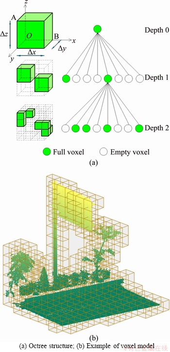
Figure 2 Voxel model:
 (3)
(3)
where di is the orthogonal distance from pi to the fitting plane, defined by the normal vector and the centroid.
3.1.2 Voxel-based region growing
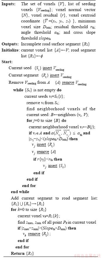
The procedure of voxel-based region growing is (herein) similar to the work of VO et al [41]. The pseudo-code is shown in Algorithm 1. However, the differences are: 1) selecting an initial seeding voxel, 2) conditions to determine the similarity between adjacent voxels, which are critical parameters affecting the segmentation results.
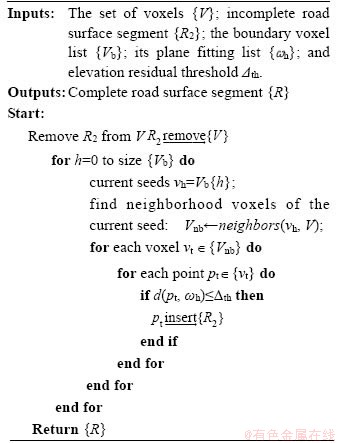
Algorithm 1 Voxel-based region growing for extracting the road surface (Step 2)
In this implementation, the seeding voxels (Vseeding) were identified as the full voxels within the road surface that have a smaller residual than the threshold. The seeding voxels were extracted from the full voxels by using the trajectory data from a mobile scanning system. The procedure of extracting the seeding voxels is as follows: 1) determine the candidate seeding voxels (Vcandidate), which solely contains the 2D trajectory data in the XY plane; 2) the seeding voxels are extracted by selecting the voxels which contain the largest number of points. The detailed procedure of extracting the seeding voxels is explained in the following section.
As the voxel model contains a large number of voxels, all full voxels need to be examined for whether they are seeding voxels or not. This requires a large computational time. This implementation extracts the initial seeding voxels as voxels on the road surface, and the segmentation process is terminated when the seeding region is empty.
Trajectory data describe locations of a vehicle during data acquisition. The projected trajectory data in the road surface were occupied by voxels representing the road surface (Figure 3). A procedure to extract initial seeding voxels started to project both the trajectory data, ptr=(xtri, ytri, ztri)R3, i=1, ��, N, where N is the total number of trajectory points, and all full voxels V onto the XY plane in the global coordinate system. The candidate seeding voxels contained the ptri to be extracted, which can be expressed in Eq. (4).

 (4)
(4)
where j=1, ��, k, where k is the total number of full voxels in the octree structure; V.xA,j, V.yA,j, V.xB,j and V.yB,j are x and y coordinates of a pair��s opposite corners (A, B) of voxel Vj.
For example, Figure 3(a) shows a point cloud and trajectory points, while the candidate initial seeding voxels are illustrated in Figure 3(b). However, many candidate seeding voxels occupy the same trajectory points (Figure 3(c)). Thus, voxels that do not represent the road surface need to be discarded. The point density of each candidate seeding voxel occupying the same trajectory was computed, and the seeding voxels were selected if they have the largest point density. The point density can be calculated based on the number of points per area of a convex hull of the horizontal projected points. This is because the road surface is below the vehicle and the point density of ground objects often are larger than those of non-ground objects [42]. For example, in Figures 3(b) and (c), although the projection of three voxels (Vcandidate6,1, Vcandidate6,2, Vcandidate6,3) occupy the trajectory points, the voxel Vcandidate6,1 is the initial seeding voxel since the voxel satisfies the above condition; the voxels Vcandidate6,2, Vcandidate6,3 are discarded (Figure 3(d)).
As the road surface is generally smooth and continuous, from a seeding voxel in a current region, its neighboring voxels can be grouped into the current region if they satisfy three conditions: 1) a deviation of normal vectors, 2) residual, and 3) height difference (Algorithm 1). The first two conditions are to ensure that patches of the road have similar orientation and roughness. The third condition (the height difference between the elevation of the given voxel vi and its neighboring voxel vj) is to avoid the neighboring voxels that do not represent the road surface although they satisfy the first two conditions, for example, the voxels of the road pavement. This condition is to ensure that the slope between the given voxel and its neighboring voxels is no larger than the lateral and longitudinal slopes of the road profile. This implies that the difference in elevation (|zvi-zvj|) should be smaller than the elevation threshold computed from the distance between two adjacent voxels and the maximum road slope. By employing the three aforementioned conditions, a set of voxels that represent the potential road region segment R1 are obtained (Figure 4(a)).
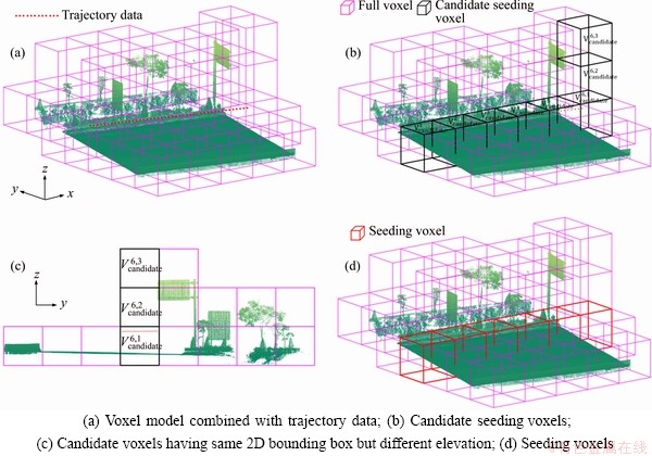
Figure 3 Result of extracting seeding voxels:
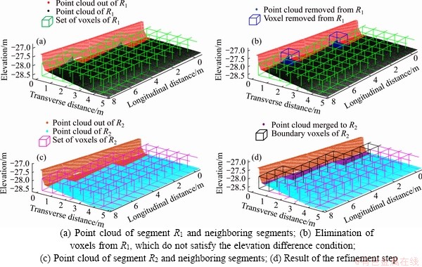
Figure 4 Voxel-based region growing:
Moreover, the voxels on the boundary of segment R1 may contain data points of a non-road surface (e.g., the voxels contain points of the road surface and pavement/footpath). This case can occur when there are non-road surface points as a small percentage of the total points within the voxel, and the features of the voxel are determined by the road surface points. Thus, these voxels must be removed from R1 (Figure 4(b)). The height difference (��H=|zmax-zmin|) between the highest and lowest elevation point in each voxel of R1 is calculated. If the height difference is higher than the height threshold computed from the maximum road slope and voxel size, the voxels are eliminated from the current region. Finally, a set of voxels which contains only the road surface points was generated from the potential road region, to form the road surface segment R2. However, it can be seen that the road boundary of segment R2 zig-zags or is incomplete (Figure 4(c)). Thus, a refinement step must be implemented to improve the boundary of the road.
3.1.3 Road surface refinement
Step 3 refines the boundaries of the road surface segment and extracts additional road surface points around the road boundary. This process merges the road surface points of other regions adjacent to the incomplete road surface segment, R2 (Algorithm 2).
The refinement process used the boundary voxels (Vb) of R2, which are voxels having less than 8 neighboring voxels belonging to R2 (Figure 4(d)). Each voxel vh��Vb was used to find the neighboring voxels (Vnb) from the remaining voxels that were not present in the set of voxels, R2. To extract the additional points of the road surface, if any point pt��Vnb has a distance to a fitting surface of vh less than the distance threshold ��th, the point pt was considered as an additional point. By employing this process, the road surface points that belong to the removable voxels in the previous step were also extracted and merged to the road surface segment, R2. The result of the refinement process is shown in Figure 4(d). Note that the distance threshold ��th was chosen based on an accumulation of two parameters: 1) the noise level of the laser scanning data and 2) the different height between the road surface and the sidewalk, which can be varied from 10 to 20 cm [43].
Algorithm 2 Road surface refinement (Step 3)
Figures 5(a) and (d) demonstrate the processes of the voxel-based road surface extraction method. Figure 5(a) shows the point cloud data, where points are shown in height color fashion. After applying the voxel-based region growing using the three above-mentioned conditions, the incomplete road surface segment R1 was determined, which is shown in Figure 5(b). Using the height difference condition, the incomplete road surface segment R2 is generated (Figure 5(c)). Finally, the complete extracted road surface is obtained by employing the refinement step (Figure 5(d)).
3.2 Application of road surface extraction: Road roughness
One of the applications based on the spatial information of the extracted road surface��s point cloud (3D coordinates) is to determine a road roughness, which is referred to as the irregularities of the surface along a longitudinal direction of the road profile [43]. There are two main types of road roughness: dynamic and static [44]. Dynamic approaches evaluate the dynamic reaction of the vehicle, while static approaches assess the road geometry directly from the road elevation profile.
For dynamic approaches, the international roughness index (IRI) is a representative of the continuous roughness of the road, which is widely used in many countries, e.g., USA. In contrast, in the static roughness approaches, the standard deviation (SD) may be used as the value of the discrete roughness of the road profile, which is commonly used in Japan. In this paper, the static road roughness in the form of the SD value was computed directly from the road elevation profile, which can be obtained from the 3D point cloud of the road surface.
According to the Japan Road Association [43], the road roughness at each road section is calculated as the SD of elevation deviations of data points within a 1.5 m interval spacing along the longitudinal road profile. The measurement of each road section (Figure 6, was performed for a road length of 100 m. The calculation of the standard deviation is obtained as the following equation:
 (5)
(5)
 (6)
(6)
where di denotes the elevation deviation at the measured location; hi�C1, hi and hi+1 are the elevations at three continuous points measured by a laser profilometer (length of 3.0 m); and n is the total number of measured points.
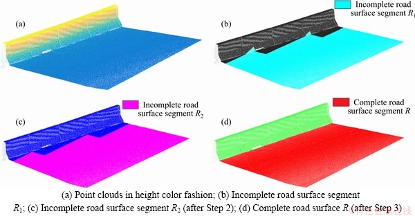
Figure 5 Result of road surface extraction:
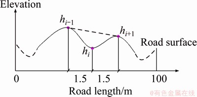
Figure 6 Longitudinal roughness measurement of road surface (JRA, 1989)
Road roughness estimation can be implemented using the elevation information from lidar data. DIAZ et al [45] used the MLS data to estimate the surface roughness in agricultural soil. From the raw point cloud data, a surface grid model with 1 cm spacing was constructed to assess the surface roughness. ZHANG et al [46] applied a multi-scale variance method to estimate the surface roughness from the point cloud collected by a mobile robotic system consisting of a laser scanner and a 2D camera. Linear-least-square regression was used to eliminate the outliers from the sample data before the variance was computed for each dataset, which is referred to as the surface roughness. A linear regression model was employed to fit the plane containing all point clouds obtained from MLS [47] or ALS [48, 49]. Then, the road roughness was estimated by calculating the SD of the elevation deviation of each point to the fitting plane. ALHASAN et al [50] proposed a method to determine the road roughness using lidar data collected by terrestrial laser scanning. A surface grid with a size of 10 cm was first created from lidar data. Then, the quarter-car model simulation was used to translate a set of longitudinal grid input data into a discrete roughness index. However, these past approaches may not provide an accurate fitting plane when the fitting plane of the road surface contains some outlier lidar points or the fitting plane does not describe an ideal road surface.
Our framework for the estimation of road roughness along a longitudinal road profile involves the following steps (Figure 7):
1) Road surface clustering (Step 1): A median strip or center divider separated the expressway into two opposite directions of traffic. Thus, the point cloud of each direction must be separated, which was done by cell-based region growing. In this process, the 3D road surface��s points were first projected onto the XY plane to create a new set of 2D points. The quadtree representation [51] was then used to recursively subdivide the initial 2D bounding box enclosing the point clouds of the road surface into smaller cells. The region growing started from any arbitrary full cell to iteratively search adjoining full cells, and all adjoining full cells can be assembled into the current cluster. The process was finished when all full cells were examined. Finally, a set of clusters containing all adjoining cells was obtained. In this implementation, the cell size (d) was chosen to ensure that there were empty cells between two adjacent road directions. Thus, d should be less than half of the smallest width of the center divider/median strip. Figure 8(a) shows the extracted road surface, which is obtained by proposed method in Section 3.1. Employing cell-based region growing, the point clouds of three clusters representing the road surface of three traffic directions are shown in Figure 8(b).
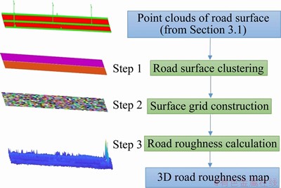
Figure 7 Framework for estimating road roughness from MLS point cloud data
2) Surface grid construction (Step 2): Next, the grid cell was constructed for the point cloud of each lane or traffic direction, in which the cell dimensions represent the footprint of the MLS vehicle��s wheels of 0.215 and 0.18 m [52]. Each cell was defined by coordinates (xc, yc, zc) where (xc, yc) are the centroid of each cell, and zc represents the standard deviation of each cell. Each road cluster was first laterally partitioned into a set of continuous small straight lateral grids with a length of 0.215 m along the longitudinal road using the trajectory data. Then, each lateral grid was longitudinally divided into a set of grid cells with dimensions of 0.215 m��0.18 m. Figure 8(c) shows an illustration of lateral grid construction for each cluster using the trajectory data. The road surface grid cell is displayed in Figure 8(d).
3) Road roughness calculation (Step 3): PCA was employed to fit a planar surface through the point cloud within each cell, in which a normal vector of the fitting surface was the eigenvector corresponding to the smallest eigenvalue derived from the covariance matrix (Eq. (2)). Next, the orthogonal distance from the points to the fitting surface was computed. Finally, the standard deviation of each cell was computed using Eq. (6), which was based on an assumption that the fitting plane in each cell describes an ideal road surface. In Eq. (6), di denotes the elevation deviation of each point in each grid, and n is the total number of data points in each cell.
This method provides the 3D road roughness map where the (x, y) coordinates are originally the centroid of each cell, and z represents the roughness of each cell position.
4 Experiments and discussion
4.1 Test sites
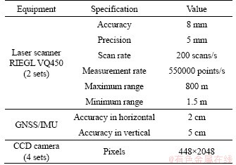
A 3D point cloud of two congested expressways in Bangkok, Thailand was collected using the GT�C4 MLS system developed by Aero Asahi Corp., Japan [53]. The MLS system contains 4 main components including 2 laser scanners (RIEGL VQ450), Global Positioning System (GPS), 360�� cameras, and Inertial Measurement Unit (IMU). The summarized technical specifications are shown in Table 1. The laser scanner can capture objects of up to 800 m with a frequency of about 550 kHz [54].
Data collection was performed with two passes (inbound and outbound) for each direction, with an average speed of 50 km/h. These designated scans were to ensure that the typical expressway components, e.g., facilitates, street, curbs, parapet, tree, guardrail, were completely captured. Site 1, at about 1.01 km of the Bang Na elevated expressway, was scanned with a total of 14056306 data points, which translates into an average point density of 560 pts/m2 (Figure 9). Site 2, at about 2.1 km including the cable-stayed Rama IX bridge, was captured with 33246417 points (659 pts/m2)(Figure 10). Notably, the terrain of Site 1 was quite flat (Figure 9(a)), while the elevation variation at Site 2 is about 49 m (Figure 10(a)).
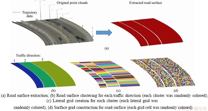
Figure 8 Framework for estimation of road roughness:
Table 1 GT�C4 specifications [54]
4.2 Parameter settings
In this study, a voxel size (Dmin) of 2 m was selected, which is less than half of the smallest width of the traffic direction (i.e., 6.2 m is the smallest width of one traffic direction at Site 1). This selection is to ensure that there is at least one voxel that contains only a point cloud of the road surface in a lateral direction, which can be used as an initial seeding voxel for voxel-based region growing.
Moreover, there are 3 thresholds: the slope (slopeth), the angle (��th), and the residual (rth). The slope threshold was determined based on the maximum value of the lateral and longitudinal slope of the road. The lateral slope of the expressway commonly varied from 2.5% to 4% [43, 55], while the maximum longitudinal slope of 5% was obtained from the construction drawing for Site 2 (Rama IX Bridge). Thus, the slope threshold (slopeth) was chosen as 5% in this study. The angle threshold was selected based on the angle between two normal vectors of two consecutive voxels (vi and vj). Considering the two-sided slope of the road surface (centerline crown) on the expressway/ highway as shown in Figure 11, there are two main cases of neighboring voxels on a road surface. For Case 1 (Figure 11(a)), the two voxels are located on the same side of the road, and the angle between two normal vectors is very small (close to zero). For Case 2 (Figure 11(b)), the two voxels are located near the centerline of the road. The angle is computed as 2��tan-1(i), and is referred to as the maximum angle. Therefore, in this study, the angle threshold was chosen as 5��, which corresponds to the angle between the two normal vectors in Case 2 for i=4% (i.e., 2��tan-10.04=4.6��).
A residual threshold was chosen based on the noise level of the road surface sample data. To estimate this threshold, 30 voxels representing the road surface were randomly selected. The noise level in each voxel is the square root of the variance of the orthogonal distance from all points within the voxel to the fitting plane. Table 2 showed the residuals from Site 1 and Site 2 with a confidence interval of 95%. The residuals were (0.017��0.004) m and (0.008��0.002) m for Site 1 and Site 2, respectively, at a 95% confidence interval. Thus, a residual of 0.03 m was chosen as the residual threshold in this paper.
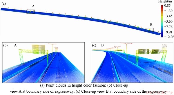
Figure 9 Point clouds of Site 1 (Bang Na elevated expressway):
Figure 10 Point clouds of Site 2 (Rama IX Bridge):
Figure 11 Two cases for angle between two neighboring voxels:
4.3 Extraction results
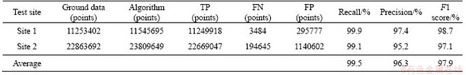
Table 3 shows threshold values and input parameters for extracting the road surface of Sites 1 and 2. The results of the extracted road surface were successfully completed for both Sites (Figures 12 and 13). A total of 11545695 and 23809649 road surface points were extracted from Site 1 and Site 2, respectively.
Table 2 Residuals for MLS data with a confidence interval of 95%
Table 3 Input parameters used for Site 1 and Site 2
The results of the proposed method were compared to the ground truth data, which were manually extracted from the data points. Although many strategies have been proposed that are point/pixel-based or object-based [56], this study employed the point-based strategy for the evaluation. That is because the road surface points significantly influence the accuracy of road geometry reconstruction. The evaluation metric involves Recall, Precision, and F1 score, which are expressed as Eqs. (7)�C(9):
 (7)
(7)
 (8)
(8)
 (9)
(9)
where TP is the extracted road surface points that belong to the ground truth; FN represents the undetected road surface points; FP denotes the extracted road surface points that were not found in the ground truth.
Figures 12(a), (d) and 13(a), (d) show the incomplete road surface R2 (after Step 2) for Site 1 and Site 2, respectively. While the complete road surface extraction is shown in Figures 12(b), (e) and 13(b), (e) (after Step 3) for Site 1 and Site 2, respectively. The ground truth data were obtained by manually extracting the point cloud of the road surface, which consists of 11253402 and 22863692 points for Site 1 and Site 2, respectively (Figures 12(c), (f) and 13(c), (f)). Results of the evaluation are shown in Table 4, where the Recall, Precision, and F1 score are respectively 99.9%, 97.4%, and 98.7% for Site 1, and 99.1%, 95.2%, and 97.1% for Site 2. This shows that the proposed algorithm extracted the data points of the road surface at Site 1 better than those at Site 2. At Site 2, the point cloud data at the road boundary in the main span of the bridge were misclassified as non-road points (under segmentation). That is because there are no noticeable height jumps at the boundary along the bridge. From Figure 13(e), the road points are located under the guardrail that was erected along the boundary of the bridge, while the road parapet was constructed along the expressway at Site 1, resulting in a significant height to separate the road surface and non-road surface (Figure 12(e)). In addition, sidewalk points at the sidewalk median strip in Site 2 were misclassified as road surface points due to the lower height difference between the roadway and the sidewalk median strip (Figure 13(e)).
The proposed algorithm was executed in the Matlab programming language [57]. The two datasets were tested on an Acer T3�C710 workstation with 2.71 GHz Intel  TM i5�C6400, and 16 GB of RAM. The execution times for Site 1 and Site 2 were about 51.2 s and 241.3 s, respectively. This shows that the proposed algorithm is feasible and efficient.
4.4 Parameter sensitivity analysis
Sensitivity analysis investigates the impact of input parameters on the road surface extraction. At each test site, we performed four different cases, corresponding to four different values of the voxel size (1, 2, 3 and 4 m). The evaluation indices, for each case are plotted (Figure 14).
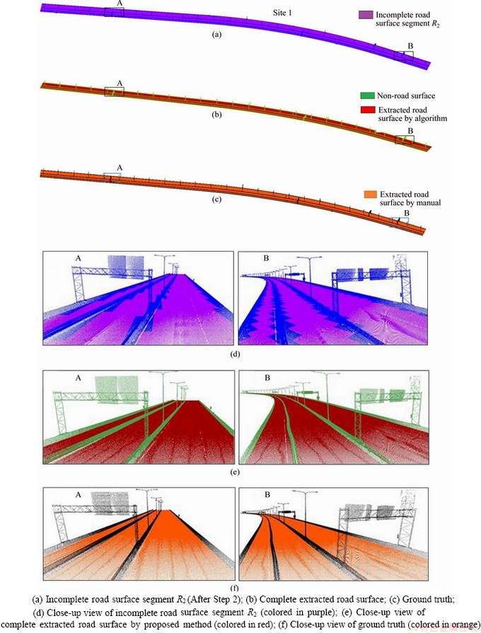
Figure 12 Stages in extraction of road surface of Site 1 (Bang Na elevated expressway):
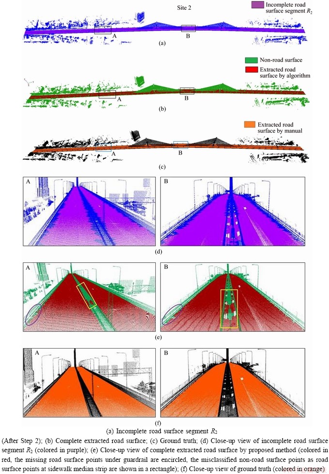
Figure 13 Stages in extraction of road surface of Site 2 (Rama IX Bridge):
Table 4 Accuracy evaluation of proposed method at two test sites
At Site 1, there was an insignificant difference in the result accuracy when the voxel size increased from 1 m to 3 m, with below 0.1% for F1 score, respectively. However, when the voxel size was changed to 4 m, a major reduction of the accuracy was obtained, in which the F1 score for the case of voxel size 4 m was significantly lower at 91.8% (Figure 14(a)). That is because the selection of voxel size is larger than half of the smallest width of the road (6.2 m at Site 1), as seen in Figures 9(b), (c). For Site 2, the larger voxel size gives less accuracy, but the difference is very little, i.e., less than 0.3% for the F1 scores (Figure 14(b)).
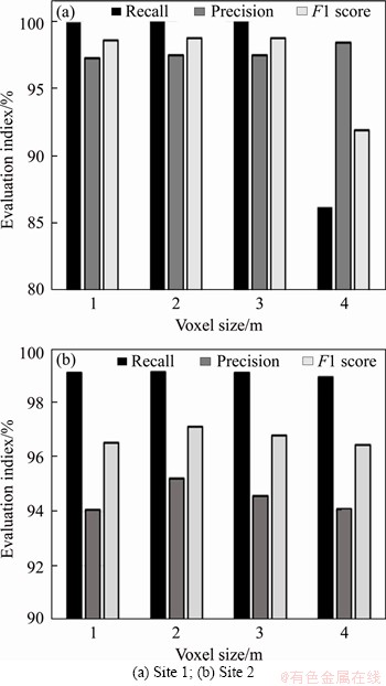
Figure 14 Sensitivity analysis of the accuracy of four different cases, corresponding to four different voxel sizes:
Based on the residuals as shown in Table 2, the values of the residual threshold (rth) range from 0.01 to 0.05 m, with an increment of 0.01 m for Site 1 and Site 2. Notably, the input parameters are used, the same as those in Table 3. From Figure 15(a), there are no discrepancies in the accuracy when the residual threshold increases from 0.03 to 0.05 m for Site 1. However, when the residual threshold decreases from 0.03 to 0.01 m, the accuracy reduces significantly. This lower accuracy is due to the higher noise level of data points at Site 1, i.e., the upper bound of the noise level is 0.021 m at the 95% confidence interval (Table 2). For Site 2, when the residual varies from 0.01 to 0.05 m, there is a small variation in the accuracy, well below 0.2% for the F1 scores (Figure 15(b)). This was due to the lower noise level of data points at Site 2 (the upper bound of the noise level is 0.010 m at a confidence interval of 95%).
Due to the variation of the lateral slope of the expressway from 2.5% to 4%, we examined three different angle threshold (��th) values of 3��, 4�� and 5��. There were no discrepancies of the accuracy for Site 1 when the angle threshold varies from 5�� to 3�� (Figure 16(a)). Similar results were also obtained at Site 2 (Figure 16(b)). The road surface slope at both sites was a one-sided slope.
The execution times corresponding to four different voxel sizes are plotted in Figure 17 for both test sites. The processing time was reduced significantly for the model using voxel sizes of 2 or 3 m when compared with those using 1 m voxel size. For example, the computing time using a 2 or 3 m voxel size was 20 times faster than the computing time using a 1 m voxel size for Site 1, while the accuracy did not change significantly. Thus, an appropriate voxel size selection was the main decision for the user in terms of accuracy and execution time.
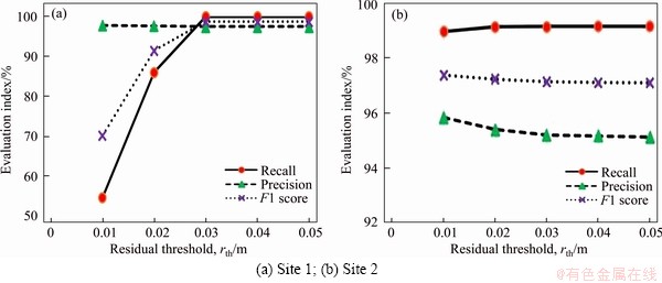
Figure 15 Sensitivity analysis of accuracy, corresponding to different residual threshold values:
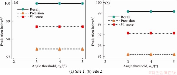
Figure 16 Sensitivity analysis of accuracy, corresponding to different angle threshold values:
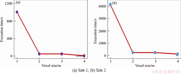
Figure 17 Execution time vs different voxel sizes:
4.5 Comparison with past studies
Comparison of the results of this proposed method with previous methods is not easy since different road environments, different point density, and accuracy of laser scanners will affect the road surface extraction results. However, a comparative analysis of the proposed method with existing methods was performed, based on the presented datasets in their studies. IBRAHIM et al [29] extracted road surface at an average detection rate of 95% and 96.53% from two datasets. YANG et al [30] presented the curb-based and scan line-based approach to extract road surface with a recall and precision of about 94.42%, and 91.13%, respectively. The average recall and precision of the extracted road boundaries are 95.41%, and 99.35%, respectively, which were also achieved by WANG et al [31]. CABO et al [32] tested their method on a 2.1 km of road, and a recall and precision of 97% and 99%, were achieved. MIYAZAKI et al [33] extracted curb points with an overall accuracy of 98%. WU et al [34] proposed a method to extract road surface in an urban street, and the detection rate from two test sites was 98.1%. The average precision and recall of the method by YANG et al [15] were about 89.6% and 96.9%, respectively. The method of YADAV et al [3] extracted the road surface at a recall of 93.8%, and a precision of 98.3%, from three test sites. The detection rate yielded 99% for extracting road surface by the approach of BALADO et al [6].
The proposed road surface extraction method in this study achieved an average recall, precision, and F1 score results are 99.5%, 96.3%, and 97.9% at the two test sites. The results showed that our method could extract road surface with a relatively high detection rate, compared with the existing methods. Moreover, most previous studies required additional data such as road spatial geometry, point density variation [29, 30], GPS time [30, 32], ordered data [30, 32, 33], road width [29], smooth road surface [33], or distance to the trajectory [31], while the proposed method uses only xyz coordinates of the unorganized point cloud as input.
4.6 Road roughness
Two road sections from the Bang Na elevated expressway were selected to demonstrate the feasibility of the framework for estimating road roughness. The first section was a six-lane road with one corridor in the middle for bidirectional traffic, covering a length of 100 m. The second road section with 200 m length had a large horizontal curve, and contained a six-lane road where opposite directions were separated by two corridors. The point clouds of road Section 1 and 2 are shown in Figures 18(a), (c), respectively.
First, a point cloud of the road surface was extracted using the proposed algorithm in Section 3.1 (Figures 18(b), (d)). According to the proposed framework, the road roughness maps were plotted for Sections 1 and 2, respectively (Figures 19 and 20). In this study, cell size (d) to group a cluster in the developed cell-based region growing algorithm was chosen as 0.3 m, for both Section data. The value of d is selected based on the width of the center divider. Figure 19 showed that the value of standard deviation varied from 1.8 to 3.1 mm for Section 1, except at the expansion joint, where the bump was seen clearly at this location with the sudden change in the value of the roughness. Similar trends were also observed in Section 2. The close-up views of the expansion joint on the expressway (Figures 19(a) and 20(a)) from roughness map at both Sections were displayed and benchmarked against the visual image (Figures 19(b), 20(b), and 20(c)). The visualization results showed that the roughness map at the location of the expansion joint is well matched with the visual image. It indicated that the proposed framework provided a high potential solution for the estimation of longitudinal road surface roughness.
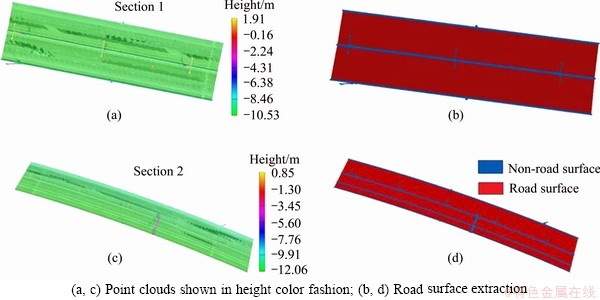
Figure 18 Three-dimensional view of Sections 1 and 2:
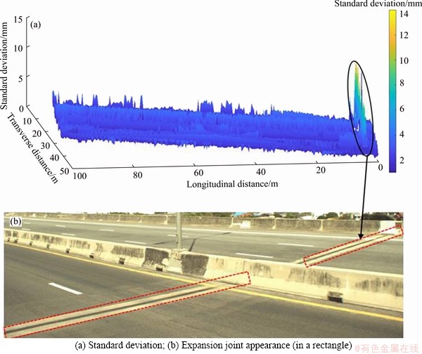
Figure 19 Roughness map of Section 1:
5 Conclusions
This paper introduces a voxel-based region growing method for automatic extraction of the road surface in an expressway environment from point cloud data collected by MLS. If there is a road curb along the road (which is noticeable on all expressways in an urban environment), the voxel-based and curb-based segmentation algorithm can extract the road surface from the large point cloud in the expressway area. The proposed method consists of three steps: (1) a voxel model was constructed from 3D point cloud data; (2) the voxel-based segmentation algorithm was applied to extract the road surface; (3) the curb-based segmentation algorithm was employed for road surface refinement. Two test sites that included flat and bumpy roads with a high slope were then used to assess the efficiency of the proposed method. The average Recall, Precision, and F1 score results are 99.5%, 96.3%, and 97.9% at the two test sites. This shows that the proposed algorithm is a reliable, robust, and automatic method to extract a road surface at high accuracy. The proposed method uses only xyz coordinates of the point cloud. This is appropriate for other datasets. In addition, our method is effective for both straight and curved road sections. Based on the extracted road surface, a framework for the estimation of road roughness was presented. The road roughness deviation map was generated successfully for two different road sections. In comparison with the methods in the literature, this proposed framework can provide spatial pavement roughness��s map with roughness indices both transversely and longitudinally. Thus, it provides more details on the localized roughness feature over conventional pavement roughness estimation method. The results demonstrated that the road roughness at the expansion joint was consistent with the visual image. It automatically outlined the road roughness map, which can be monitored and assessed by maintenance infrastructure authorities, to improve the quality of a road surface.
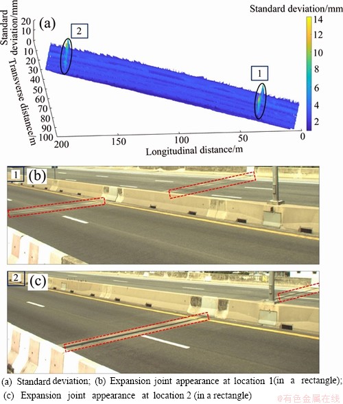
Figure 20 Roughness map of Section 2:
References
[1] GUAN H, LI J, YU Y, CHAPMAN M, WANG C. Automated road information extraction from mobile laser scanning data [J]. IEEE Transactions on Intelligent Transportation Systems, 2015, 16(1): 194-205. DOI:10.1109/TITS.2014.2328589.
[2] DAVIES R B, CENEK P D, HENDERSON R J. The effect of skid resistance and texture on crash risk [C]// International Conference on Surface Friction�CRoads and Runways. Christchurch, New Zealand, 2005.
[3] YADAV M, SINGH A K, LOHANI B. Extraction of road surface from mobile lidar data of complex road environment [J]. International Journal of Remote Sensing, 2017, 38(16): 4655-4682. DOI:10.1080/01431161.2017.1320451.
[4] SOILAN M, TRUONG H L, RIVEIRO B, LAEFER D. Automatic extraction of road features in urban environments using dense ALS data [J].International Journal of Applied Earth Observation and Geoinformation, 2018,64: 226-236. DOI: 10.1016/j.jag.2017.09.010.
[5] ALSHEHHI R, MARPU P R. Hierarchical graph-based segmentation for extracting road networks from high-resolution satellite images [J]. ISPRS Journal of Photogrammetry and Remote Sensing, 2017,126:245-260. DOI: 10.1016/j.isprsjprs.2017.02.008.
[6] BALADO J, DIAZ-VILARINO L, ARIAS P, GONZALEZ- JORGE H. Automatic classification of urban ground elements from mobile laser scanning data [J].Automation in Construction, 2018, 86: 226-239. DOI: 10.1016/j.autcon. 2017.09.004.
[7] MA L, LI Y, LI J, WANG C, WANG R, CHAPMAN M A. Mobile laser scanned point-clouds for road object detection and extraction: A Review [J].Remote Sensing, 2018,10(10): 1531. DOI:10.3390/rs10101531.
[8] CHEN De-liang, HE Xiu-feng. Fast automatic three-dimensional road model reconstruction based on mobile laser scanning system [J]. Optik, 2015, 126: 725-730. DOI: 10.1016/j.ijleo.2015.02.021.
[9] AKAGUL M, YURTSEVEN H, AKBURAK S, DEMIR M, CIGIZOGLU H K, OZTURK T, EKSI M, AKAY A O. Short term monitoring of forest road pavement degradation using terrestrial laser scanning [J]. Measurement, 2017, 103: 283- 293. DOI: 10.1016/j.measurement.2017.02.045.
[10] YANG MM, WAN Y C, LIU X L, XU J Z, WEI Z Y, CHEN M L, SHENG P. Laser data based automatic recognition and maintenance of road markings from MLS system [J]. Optics & Laser Technology, 2018, 107: 192-203. DOI: 10.1016/ j.optlastec.2018.05.027.
[11] YAO L, CHEN Q, QIN C, WU H, ZHANG S. Automatic extraction ofroadmarkings from mobilelaser-point cloud using intensity data [C]// International Archives of the Photogrammetry, Remote Sensing and Spatial Information Sciences. Beijing, China, 2018: 2113-2119.
[12] GUAN H, YAN W, YU Y, ZHONG L, LI D. Robust traffic-sign detection and classification using mobile Lidar data withdigital images [J]. IEEE Journal of Selected Topics in Applied Earth Observation and Remote Sensing, 2018, 11(5): 1715-1724. DOI: 10.1109/JSTARS.2018.2810143.
[13] GEHRUNG J, HEBEL M, ARENS M, STILLA U. An approach to extract moving objects from MLS data using a volumetric background representation [C]//ISPRS Annals of the Photogrammetry, Remote Sensing and Spatial Information Sciences. Hannover, Germany, 2017. DOI: 10.5194/isprs-annals-IV-1-W1-107-2017.
[14] YADAV M, SINGH A K. Rural road surface extraction using mobile LiDAR point cloud data [J]. Journal of the Indian Society of Remote Sensing, 2018, 46(4): 531-538. DOI: 10.1007/s12524-017-0732-4.
[15] YANG B, LIU Y, DONG Z, LIANG F, LI B, PENG X. 3D local feature BKD to extract road information from mobile laser scanning point clouds [J]. ISPRS Journal of Photogrammetry and Remote Sensing, 2017, 130: 329-343. DOI: 10.1016/j.isprsjprs.2017.06.007.
[16] ZAI D W, LI J, GUO Y L, CHENG M, LIN Y B, LUO H, WANG C. 3-D road boundary extraction from mobile laser scanning data via supervoxels and graph cuts [J]. IEEE Transactions on Intelligent Transportation Systems, 2018, 19(3): 802-813. DOI: 10.1109/TITS.2017.2701403.
[17] XU S, WANG R, ZHENG H. Road curb extraction from mobile LiDAR point clouds [J]. IEEE Transactions on Geoscience and Remote Sensing, 2017, 55(2): 996-1009. DOI: 10.1109/TGRS.2016.2617819.
[18] KUMAR P, LEWIS P, MCCARTHY T. The potential of active contour models in extractingroad edges from mobile laser scanning data [J].Infrastructures, 2017, 2(3): 9. DOI: 10.3390/infrastructures2030009.
[19] NEUPANE S R, GHARAIBEH N G. A heuristic-based method for obtaining road surface type information from mobile lidar for use in network-level infrastructure management [J].Measurement, 2019, 131: 664-670. DOI: 10.1016/j.measurement.2018.09.015.
[20] HOLGADO-BARCO A, RIVEIRO B, GONZALEZ- AGUILERA D, ARIAS P. Automatic inventory of road cross-sections from mobilelaser scanning system [J]. Computer-Aided Civil and Infrastructure Engineering, 2017, 32(1): 3-17. DOI: 10.1111/mice.12213.
[21] CHENG M, ZHANG H, WANG C, LI J. Extraction and classification of roadmarkings using mobile laser scanning point clouds [J]. IEEE Journal of Selected Topics in Applied Earth Observation and Remote Sensing, 2017, 10(3): 1182-1196. DOI: 10.1109/JSTARS.2016.2606507.
[22] LI F, ELBERINK S O, VOSSELMAN G. Pole-like road furniture detection and decomposition in mobile laser scanning data based on spatial relations [J]. Remote Sensing, 2018, 10 (4): 531. DOI: 10.3390/rs10040531.
[23] LI Y, WANG W X, TANG S J, LI D L, WANG Y K, YUAN Z L, GUO R Z, LI X M, XIU W Q. Localization and extraction of road poles in urban areas from mobile laser scanning data [J]. Remote Sensing, 2019, 11(4): 401. DOI: 10.3390/ rs11040401.
[24] CHEN S, TRUONG-HONG L, LAEFER D F, MANGINA E. Automated bridge deck evaluation through UAV derived point cloud [C]// CERI2018 Congress. The 2018 Civil Engineering Research in Ireland Conference. Dublin: CERAI, 2018: 735-740.
[25] KARILA K, MATIKAINEN L, PUTTONEN E, HYYPPA J. Feasibility of multispectral airborne laser scanning data for road mapping [J]. IEEE Geoscience and Remote Sensing Letters, 2017, 14(3): 294-298. DOI: 10.1109/LGRS.2016. 2631261.
[26] MATIKAINEN L, KARILA K, HYYPPA J, LITKEY P, PUTTONEN E, AHOKAS E. Object-based analysis of multispectral airborne laser scanner data for land cover classification and map updating [J]. ISPRS Journal of Photogrammetry and Remote Sensing, 2017, 128: 298-313. DOI: 10.1016/j.isprsjprs.2017.04.005.
[27] MCELHINNEY C, KUMAR P, CAHALANE C, MCCARTHY T. Initial results from european road safety inspection (EURSI) mobile mapping project [C]// International Archives of the Photogrammetry, Remote Sensing and Spatial Information Sciences. Newcastle, UK, 2010.
[28] ZHANG W. Lidar based road and road-edge detection [C]// Proceedings of IEEE Intelligent Vehicles Symposium. San Diego, USA, 2010. DOI: 10.1109/IVS.2010.5548134.
[29] IBRAHIM S, LICHTI D. Curb-based street floor extraction from mobile terrestrial lidar point cloud [C]// International Archives of the Photogrammetry, Remote Sensing and Spatial Information Sciences. Melbourne, Australia, 2012. DOI: 10.5194/isprsarchives-XXXIX-B5-193-2012.
[30] YANG B, FANG L, LI J. Semi-automated extraction and delineation of 3d roads of street scene from mobile laser scanning point clouds [J]. ISPRS Journal of Photogrammetry and Remote Sensing, 2013, 79: 80-93. DOI: 10.1016/ j.isprsjprs.2013.01.016.
[31] WANG H Y, LUO H, WEN C L, CHENG J, LI P, CHEN Y P, WANG C, LI J. Road boundary detection based on local normal saliency from mobile laser scanning data [J]. IEEE Geoscience and Remote Sensing Letters, 2015, 12(10): 2085-2089. DOI: 10.1109/LGRS.2015.2449074.
[32] CABO C, KUKKO A, GARCIA-CORTES S, KAARTINEN H, HYYPPA J, ORDONEZ C. An algorithm for automatic road asphalt edge delineation from mobile laser scanner data using the line clouds concept [J]. Remote Sensing, 2016, 8(9): 1-20. DOI: 10.3390/rs8090740.
[33] MIYAZAKI R, YAMAMOTO M, HANAMOTO E, IZUMI H, HARADA K. A line-based approach for precise extraction of road and curb region from mobile mapping data [C]// ISPRS Annals of Photogrammetry, Remote Sensing and Spatial Information Sciences. Rivar del Garda, Italy, 2014. DOI: 10.5194/isprsannals-II-5-243-2014.
[34] WU B, YU B, HUANG C, WU Q, WU J. Automated extraction of ground surface along urban roads from mobile laser scanning point clouds [J]. Remote Sensing Letters, 2016, 7(2): 170-179. DOI: 10.1080/2150704X.2015. 1117156.
[35] RUSU R B, MARTON Z C, BLODOW N, DOLHA M, BEETZ M. Towards 3D point cloud based object maps for household environments [J]. Robotics and Autonomous System, 2008, 56(11): 927-941. DOI: 10.1016/j.robot.2008. 08.005.
[36] CloudCompare. GNU general public license, Version 2.10. [EB/OL]. http://www.cloudcompare.org/.
[37] AYALA D, BRUNET P, JUAN R, NAVAZO I. Object representation by means of nominal division quadtrees and octrees [J]. ACM Transactions on Graphics, 1985, 4(1): 41-59. DOI: 10.1145/3973.3975.
[38] WANG J, OLIVEIRA M M, XIE H, KAUFMAN A E. Surface reconstruction using oriented charges [C]// Proceeding of Computer Graphics. Stony Brook, NY, USA, 2005. DOI:10.1109/CGI.2005.1500390.
[39] PULLI K, DUCHAMP T, HOPPE H, MCDONALD J, SHAPIRO L, STUETZLE W. Robust meshes from multiple range maps [C]// International Conference on Recent Advances in 3-D Digital Imaging and Modeling. Ottawa, Ontario, Canada, 1997. DOI: 10.1109/IM.1997.603867.
[40] HOPPE H, DEROSE T, DUCHAMP T, MCDONALD J, STUETZLE W. Surface reconstruction from unorganized points [C]// Proceedings of the 19th Annual Conference on Computer Graphics and Interactive Techniques (SIGGRAPH), 1992. DOI: 10.1145/142920.134011.
[41] VO A V, HONG L T, LAEFER D F, BERTOLOTTO M. Octree-based region growing for point cloud segmentation [J]. ISPRS Journal of Photogrammetry and Remote Sensing, 2015, 104: 88-100. DOI: 10.1016/j.isprsjprs.2015.01.011.
[42] ARMESTO J, PARDINAS R J, LORENZO H, ARIAS P. Modelling masonry arches shape using terrestrial laser scanning data and nonparametric methods [J]. Engineering Structures, 2010, 32(2): 607-615. DOI: 10.1016/j.engstruct. 2009.11.007.
[43] JRA-Japan Road Association. Manual for asphalt pavement [M]. Tokyo, Japan, 1989.
[44] FARIAS M M, SOUZA R O. Correlations and analyses of longitudinal roughness indices [J]. Road Materials and Pavement Design, 2009, 10(2): 399-415. DOI: 10.1080/ 14680629.2009.9690202.
[45] DIAZ J C F, JUDGE J, SLATTON K C, SHRESTHA R, CARTER W E, BLOOMQUIST D. Characterization of full surface roughness in agricultural soils using ground based LiDAR [C]// Proceeding of IEEE International Geoscience and Remote Sensing Symposium (IGARSS). Honolulu, Hawaii, USA, 2010. DOI: 10.1109/IGARSS.2010.5652056.
[46] ZHANG A M, RUSSELL R A. Surface roughness measurement for outdoor mobile robotic applications [C]// Proceedings of Australasian Conference on Robotics and Automation. Canberra, Australia, 2004.
[47] YEN K S, AKIN K, LOFTON A, RAVANI B, LASKY T A. Using mobile laser scanning to produce digital terrain models of pavement surfaces [R]. California Department of Trans Portation: CA10-1113. http://ahmct.ucdavis.edu/ pdf/UCD-ARR-10-11-30-01.pdf.
[48] PATTNAIK S B, HALLMARK S, SOULEYRETTE R. Collecting road inventory using LIDAR surface models [C]// Proceedings of Map India Conference. New Delhi, India, 2003.
[49] ZHANG K, FREY H C. Road grade estimation for on-road vehicle emissions modeling using LIDAR data [C]// Proceedings of Air & Waste Management Association Annual Meeting. Minneapolis, USA, 2005. DOI: 10.1080/10473289.2006.10464500.
[50] ALHASAN A, WHITE D J, BRABANTER K D. Spatial pavement roughness from stationary laser scanning [J]. International Journal of Pavement Engineering, 2017,18(1): 83-96.DOI: 10.1080/10298436.2015.1065403.
[51] SAMET H. The quadtree and related hierarchical data tructures [J]. ACM Computer Surveys, 1984, 16(2): 187-260. DOI: 10.1145/356924.356930.
[52] KUMAR P, LEWIS P, MCELHINNEY C P, RAHMAN A A. An algorithm for automated estimation of road roughness from mobile laser scanning data [J].Photogrammetric Record, 2015, 30(149): 30-45. DOI: 10.1111/phor.12090.
[53] MLS GT-4. Mobile mapping system GT-4 [EB/OL]. [2019-10-01]. https://www.aeroasahi.co.jp/english/equipmen t/detail.php?id=21.
[54] RIEGL VQ-450. High speed 2D laser scanner with online waveform processing [EB/OL]. [2019-05-24]. http://www. riegl.com/uploads/tx_pxpriegldownloads/10_DataSheet_VQ-450_rund_2014-09-02.pdf (accessed on 24 May 2019).
[55] EXAT�CExpressway and Rapid Transit Authority of Thailand. Expressway inspection manual and maintenance procedure [M]. Bangkok, Thailand, 2006.
[56] TRUONG-HONG L, LAEFER D F. Quantitative evaluation strategies for urban 3D model generation from remote sensing data [J].Computer & Graphics, 2015,49: 82-91.DOI: 10.1016/j.cag.2015.03.001.
[57] The MathWorks. MATLAB function reference [M]. The Mathwork, 2007.
(Edited by HE Yun-bin)
���ĵ���
���ٹ�··���ƶ�����ɨ�����ݵ��Զ���ȡ
ժҪ�������һ�ֻ�������������������������ڸ��ٹ�·�������ƶ�����ɨ����Ƶ�·���Զ���ȡ���÷�������������Ҫ����: ��������ģ��; ���û������صķָ��㷨��ȡ·���; ���û��ڱ߽�ķָ��㷨ϸ����·�߽硣Ϊ�����۸÷�����ȷ�ԣ�����ʹ���˸��ٹ�·ƽ̹�͵�������·�滷���µ������������������������ݼ������㷨�ɹ���ʵ����·��ĸ߾�����ȡ��ƽ���ٻ���Ϊ99.5%������Ϊ96.3%��F1�÷�Ϊ97.9%����������ȡ��·�棬�����һ��·��ƽ���ȹ��ƿ�ܡ�����·��ֲڶ�ͼ�Ľ�����Ӿ�ͼ����бȽ�ʱ���õ��˺ܺõ�һ���ԣ�˵���������ܵĿ����Ժ���Ч�ԡ�
�ؼ��ʣ��ƶ�����ɨ��; �ָ�; ·��; ���ٹ�·; ���ػ�; ����
Foundation item: Project(SIIT-AUN/SEED-Net-G-S1 Y16/018) supported by the Doctoral Asean University Network Program; Project supported by the Metropolitan Expressway Co., Ltd., Japan; Project supported by Elysium Co. Ltd.; Project supported by Aero Asahi Corporation, Co., Ltd.; Project supported by the Expressway Authority of Thailand
Received date: 2019-06-24; Accepted date: 2020-05-07
Corresponding author: TRAN Thanh Ha, PhD Candidate; Tel: +66-953274390; E-mail: thanhhabk2006@gmail.com; ORCID: 0000- 0001-5175-0547
Abstract: This paper presents a voxel-based region growing method for automatic road surface extraction from mobile laser scanning point clouds in an expressway environment. The proposed method has three major steps: constructing a voxel model; extracting the road surface points by employing the voxel-based segmentation algorithm; refining the road boundary using the curb-based segmentation algorithm. To evaluate the accuracy of the proposed method, the two-point cloud datasets of two typical test sites in an expressway environment consisting of flat and bumpy surfaces with a high slope were used. The proposed algorithm extracted the road surface successfully with high accuracy. There was an average recall of 99.5%, the precision was 96.3%, and the F1 score was 97.9%. From the extracted road surface, a framework for the estimation of road roughness was proposed. Good agreement was achieved when comparing the results of the road roughness map with the visual image, indicating the feasibility and effectiveness of the proposed framework.
