
J. Cent. South Univ. (2012) 19: 615-622
DOI: 10.1007/s11771-012-1047-9![]()
Characteristics of ventilation coefficient and its impact on urban air pollution
LU Chan(·�), DENG Qi-hong(������), LIU Wei-wei(��εΡ), HUANG Bo-liang(�ư���), SHI Ling-zhi(ʯ��֥)
School of Energy Science and Engineering, Central South University, Changsha 410083, China
? Central South University Press and Springer-Verlag Berlin Heidelberg 2012
Abstract:
The temporal variation of ventilation coefficient was estimated and a simple model for the prediction of urban ventilation coefficient in Changsha was developed. Firstly, Pearson correlation analysis was used to investigate the relationship between meteorological parameters and mixing layer height during 2005-2009 in Changsha, China. Secondly, the multi-linear regression model between daytime and nighttime was adopted to predict the temporal ventilation coefficient. Thirdly, the validation of the model between the predicted and observed ventilation coefficient in 2010 was conducted. The results showed that ventilation coefficient significantly varied and remained high during daytime, while it stayed relatively constant and low during nighttime. In addition, the diurnal ventilation coefficient was distinctly negatively correlated with PM10 (particle with the diameter less than 10 ��m) concentration in Changsha, China. The predicted ventilation coefficient agreed well with the observed values based on the multi-linear regression models during daytime and nighttime. The urban temporal ventilation coefficient could be accurately predicted by some simple meteorological parameters during daytime and nighttime. The ventilation coefficient played an important role in the PM10 concentration level.
Key words:
ventilation coefficient; mixing layer height; particulate matter; multi-linear regression��
1 Introduction
Air pollution is a serious problem attracting much attention all over the world. Identifying the source of air pollution is essential to determine atmospheric pollution, meanwhile effective control has been emphasized in recent studies. Consideration must be given to meteorological parameters influencing urban air pollution [1-2]. However, the studies regarding these problems have been limited until now.
The two most important meteorological parameters are: the mixing layer height (MLH) and wind speed [3-5]. The mixing layer height indicates the vertical diluted ability of air pollutants, and the wind speed represents the horizontal ventilation, which benefits the dispersion of air pollution. Therefore, the ventilation coefficient, which is a product of mixing layer height multiplied by average wind speed, implies the assimilative potential and ventilation capacity [6-7]. The ventilation coefficient plays an important role in the dilution and elimination of aerosols, and can be considered as one of the factors determining pollution potential over a region of interest. Some studies [8-11] have investigated the characteristics of the ventilation coefficient. For example, GOYAL and CHALAPATI [7] investigated the temporal characteristic of the ventilation coefficient in Kochi, and they stated that the ventilation coefficient was higher during the afternoon, while it was lower during the evening and morning in all the seasons. In addition, the study by MANJU et al [12] in Manali demonstrated that the highest ventilation coefficient between 13:00 and 16:00 implied potentially safe hours for dispersion of the pollutants during summer. However, most of these studies only aimed at the characteristics of ventilation coefficient but did not focus on the relationship between ventilation coefficient and air pollution.
China is the biggest developing country with urban intensively increasing air pollution due to the rapid development of urbanization, basic constructions and economic development, which exerts an adverse effect on the urban environment, health and climate change. To date, the air pollution in China has attracted much attention around the world. The most serious air pollution is mainly distributed in the large and medium cities, especially the capital cities. Changsha, the capital city of Hunan province, is located at the central south of China. Similar to other capital cities, Changsha has experienced increasing air pollution attributed to urban industrialization and basic construction, which posed a potential threat to the entire city. Changsha belongs to the subtropical monsoon climate, and consequently its meteorological parameters (temperature, wind speed and relative humidity) intensively vary during the whole year. However, such climatic disadvantage may create an uncertain risk on the air quality. Therefore, it is of significant importance to investigate the impact of the meteorological conditions on the urban air pollution in Changsha, China.
PM10 (particle with the diameter less than 10 ��m), as one of the most important air pollutants, can be greatly influenced by the meteorological condition. PM10 pollution in Changsha is relatively serious due to the intensive basic construction and the specific climate characteristics. Thereby, urban ventilation coefficient can be regarded as an important standard of urban ventilation and assimilative pollution ability.
To better estimate the ventilation coefficient and to further understand its association with air pollution, a large amount of studies [13-20] have practiced different methods to measure the mixing layer height such as Lidar observation, numerical experiment (MM5), simple diagnostic model (AERMET), profiler-derived CBL height, ultra high frequency (UHF) wind profiler, and lapse adiabatic line. However, as the costly expenditure and restriction in time and frequency, it is extraordinarily intricate and unfeasible to be implemented. Besides, sometimes, the results incline to be imprecise in this way probably attributed to the handicaps during measurement and uncertainty of some parameters in the models. In consequence, this work provides an easier and less expensive alternative method to calculate the temporal ventilation coefficient than other methodologies. This method provides a simple and accurate method to evaluate and predict the real time ventilation coefficient in the cities.
In this work, the temporal characteristic of urban ventilation coefficient and its quantitative relation are analyzed with meteorological parameters during daytime and nighttime, as well as its influence to PM10 level in Changsha, China. In addition, accurate multi-linear regression models are provided by some meteorological parameters for the calculation and prediction of the ventilation coefficient.
2 Method
2.1 Sample location
The railway station of Changsha was selected as the sampling location for this work. This railway station is adjacent to the downtown of Changsha. A number of activities by trains, vehicles and human beings occur at this location every day. The trains operate regularly on a 24 h schedule every day. In addition, there are two large-scale bus stations in close proximity to the railway station: one is located in the west and the other is located in the south. These local buses operate daily starting at 6:00 and continuing to 00:00 year round. Vehicular traffic by cars and motorcycles is a common phenomenon along the main traffic artery around the railway station. Also noted within the vicinity of the railway station is ongoing construction of shopping malls and residential buildings.
PM10 sampling was located on the top of a building, approximately 10 m above ground level (AGL). The PM10 sampling location was selected there because no other building or barrier was higher to possibly prevent the airflow at the sample location, which otherwise may have affected the aerosol pollution.
2.2 Data of meteorological parameters
Data of the meteorological parameters including mixing layer height (MLH), solar radiation (SR), temperature (T), pressure (Pre), relative humidity (RH), wind speed (WS), and dew point temperature (DT) on the airport of Changsha were collected from the meteorological websites during 2005-2009. The data of MLH and SR were downloaded from the website of NOAA (http://ready.arl.noaa.gov/HYSPLIT_traj.php) by HYSPLIT 4 (Hybrid Single-Particle Lagrangian Integrated Trajectory) Model. The data of T, Pre, RH, WS and DT were downloaded from the website of weather underground (http://www.wunderground.com/). The 24-hourly PM10 concentration in 2008 was obtained from Changsha Environmental Protection Bureau.
In this work, the total number of the data during 2005-2009 is 41 621, and non-precipitation cases accounts for about 86% (35 662). The data received during precipitation are excluded due to a dry-adiabatic lapse rate in the mixing layer [13]. For the main purpose of the present work, the non-precipitation data are considered adequately representative of all cases.
2.3 Calculation of ventilation coefficient
Ventilation coefficient (VC, V) is a product of mixing layer height and average wind speed through the mixing layer. The ventilation coefficient reflects the transport rate of populations in the mixing layer. The calculation of VC is given by
V=ZiU (1)
where Zi is atmospheric mixing layer height above the ground at height of i meters (m); U is average wind velocity near the ground (m/s).
In this work, the values of Zi and U were selected at height of 10 m above ground. Lower ventilation coefficient indicates less dispersion potential of pollutants in the atmosphere. The higher the coefficient is, the greater the ability of the atmosphere to disperse the pollutants is. The values of ventilation coefficient were calculated based on the data of mixing layer height and wind speed on the airport and railway station.
3 Results
3.1 Diurnal variation of ventilation coefficient in different seasons
The hourly values of the mixing layer height indicated a similar trend in all the seasons. As shown in Fig. 1, the mixing layer height increased from 8:00, and reached the maximum at 14:00 ranging from 1 471 m in summer to 949 m in winter. Then, it decreased from 14:00 till 19:00, and tended to be invariable from 20:00 to 7:00. The lowest values of the mixing layer height were equal to or less than 200 m during all the seasons. The wind speed indicated a slightly different trend compared with the mixing layer height which moderately increased from 8:00 and reached the maximum value between 14:00 and 16:00. Then, it rapidly decreased until 19:00, and lightly changed from 20:00 to 7:00. Basically, both mixing layer height and wind speed intensively varied during 8:00-19:00 and significantly high, while they nearly tended to be invariable and low during 20:00-7:00. Therefore, both of the mixing layer height and wind speed showed the same trend in the different seasons.
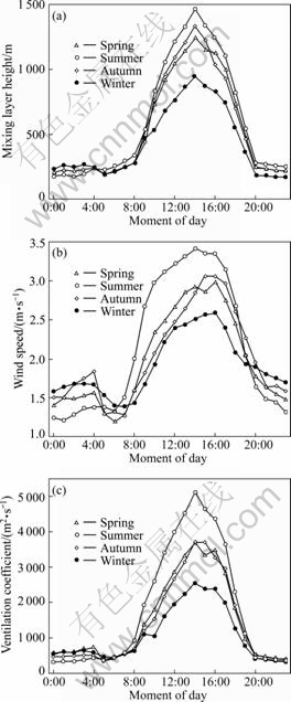
Fig. 1 Variations of hourly MLH (a), WS (b) and VC (c) in different seasons at Changsha during 2005-2009
Combined with the mixing layer height and wind speed, the ventilation coefficient showed the similar diurnal trend. The ventilation coefficient greatly varied during 8:00-19:00, while it seemed to be unalterable during 20:00-7:00. The maximum values of ventilation coefficient were 5 122 m2/s in summer followed by 3 711 m2/s in autumn and 3 694 m2/s in spring, respectively. Winter records had the smallest value of 2 537 m2/s. All the maximum values were found to occur at 14:00.
3.2 Ventilation coefficient during daytime and nighttime
Figure 2 shows the monthly variation of the mixing layer height, wind speed and ventilation coefficient during daytime and nighttime. The value of mixing layer height during daytime was greatly higher than that during nighttime, as shown in Fig. 2(a). Mean mixing layer height during daytime differed by less than 300 m in most months except for November, December and January, and the value during nighttime changed by less than 100 m in all months. Values for the daytime mixing layer height showed large variations during the year. They were the deepest of about 925-1 070 m during May through October, and the shallowest of about 600-650 m in December and January with rapid changes in transition months. Values for nighttime mixing layer height varied throughout the year by only less than 100 m. In general, the maximum nighttime occurred in July and the minimum occurred in November and December.
Average wind speeds throughout daytime and nighttime are shown in Fig. 2(b). Daytime wind speeds ranged from about 2 m/s to 3.5 m/s and nighttime wind speeds varied from about 1.2 m/s to 1.8 m/s. Like the mixing layer height, wind speed and its variation were greater during daytime than nighttime. In addition, annual variations during daytime and nighttime were different. Generally, larger speeds occurred from July to September during daytime, and during nighttime in September, October, January and February. Lower speeds commonly occurred from November to March during daytime and in May and June during nighttime.

Fig. 2 Monthly mean MH (a), WS (b) and VC (c) for daytime and nighttime at Changsha during 2005-2009
Based on the variations of mean mixing layer height and wind speed during daytime and nighttime, the ventilation coefficient varied more or less from month to month and from daytime to nighttime. Basically, the ventilation coefficient during daytime was greatly larger than that during nighttime, and mean daytime values significantly varied in different months while mean nighttime values tended to be slightly changed between different months. Figure 2(c) showed that the maxima of ventilation coefficient during daytime and nighttime were 4 264.10 m2/s and 561.64 m2/s in July, while the minimum values of them were 1 436.4 m2/s in December and 270.62 m2/s in June. It was noteworthy that in July there was a larger standard deviation of ventilation coefficient compared with other months.
3.3 Relation between ventilation coefficient and meteorological parameters
Since it was difficult to estimate the ventilation coefficient, we analyzed it by two meteorological factors: mixing layer height and wind speed, separately. However, measuring and calculating the mixing layer height were tough and complex based on the current detecting methods and experiential models. Therefore, in this work, the correlation of mixing layer height and meteorological parameters was analyzed including solar radiation (S), wind speed (W), temperature (T), pressure (P), relative humidity (HR) and dew point temperature (TD). Then, the multi-linear regression was adopted by these meteorological parameters to obtain the reasonable model of mixing layer height at daytime and nighttime during 2005-2009.
The data were separated into two time segments as daytime from 8:00 to 19:00 and nighttime from 20:00 to 7:00. Table 1 gives the correlation of mixing layer height with the meteorological parameters between daytime and nighttime. In Table 1, the mixing layer height had the largest correlation coefficient (0.799) with solar radiation during daytime, while it was mainly correlated with wind speed during nighttime (R=0.451). This result indicated the existence of different essential factors influencing the mixing layer height during daytime and nighttime, respectively. Therefore, the sun exerted significant importance on the variation of mixing layer height and hence on the ventilation coefficient during daytime, while the wind speed played an important role in the alteration of mixing layer height and hereby in the ventilation coefficient during nighttime. In addition, the mixing layer height also had relatively high correlation coefficients with relative humidity and temperature during daytime, while the relative humidity had moderately strong relation with mixing layer height during nighttime.
Table 1 Correlations of mixing layer height with meteorological parameters

Based on the correlation of mixing layer height with the meteorological parameters between daytime and nighttime, the multi-linear regression models of the mixing layer height between daytime and nighttime using the stepwise method were listed as follows:
Hdaytime=1.45S+52.84W+11.39P+54.77T-47.34TD+
9.97HR-12 530.29 (2)
Hnighttime=48.6W-2.28HR+1.86T+0.08S+0.65P-337.37 (3)
where Hdaytime and Hnighttime are the hourly mixing layer heights during daytime and nighttime.
It was noted that the partial regression coefficients of the mixing layer heights during daytime and nighttime were 0.83 and 0.49, respectively. Their combination resulted in a good coincidence between regressed and observed ventilation coefficient during the whole day with the high correlation coefficient of 0.94. As shown in Fig. 3, the seasonal correlations of diurnal predicted and observed ventilation coefficient were higher than 0.9, which interpreted good accordance between regressed and observed values. However, some hourly regressed ventilation coefficients were relatively greatly deviated from the observed values, such as the minimum regression values during 20:00-23:00 and the maximum regression values during 12:00-16:00.
3.4 Relation between ventilation coefficient and PM10 concentration
To further understand the correlation between ventilation coefficient and PM10 concentration, the railway station of Changsha was selected as one of the most seriously polluted areas to investigate the influence of ventilation coefficient on the PM10 concentration in Changsha. Four similar but different PM10 trends were detected: PM10 concentration was significantly high during night especially around 19:00, and it markedly decreased till noon. Finally, PM10 concentrations at the railway station showed an increasing trend during daytime probably due to the influence of the different and continuous anthropogenic activities as well as the variation of the ventilation coefficient. As shown in Fig. 4, the ventilation coefficient was significantly negatively correlated with PM10 concentration in different seasons. Similar to the result on the airport during 2005-2009 depicted in Section 3.1, the ventilation coefficient at the railway station was obviously high and variable during daytime, while it was low and invariable during nighttime. Accordingly, the PM10 concentration was more serious during nighttime than daytime. This may be resulted from the relatively intensive airborne pollution in the atmosphere due to the variable pollution sources including unreasonably located industries, substantive traffic emissions and some specific heavy exhaust. The contrary trend of variation between diurnal ventilation coefficient and PM10 concentration indicated that the ventilation coefficient, to a large extent, exerted an important effect on the PM10 variation in Changsha. Therefore, it is far-reaching for the local government to take some reasonable strategies to improve the urban ventilation and air quality.
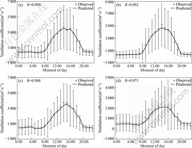
Fig. 3 Correlation between daily predicted and observed ventilation coefficient (VC) from 2005 to 2009: (a) Spring; (b) Summer; (c) Autumn; (d) Winter
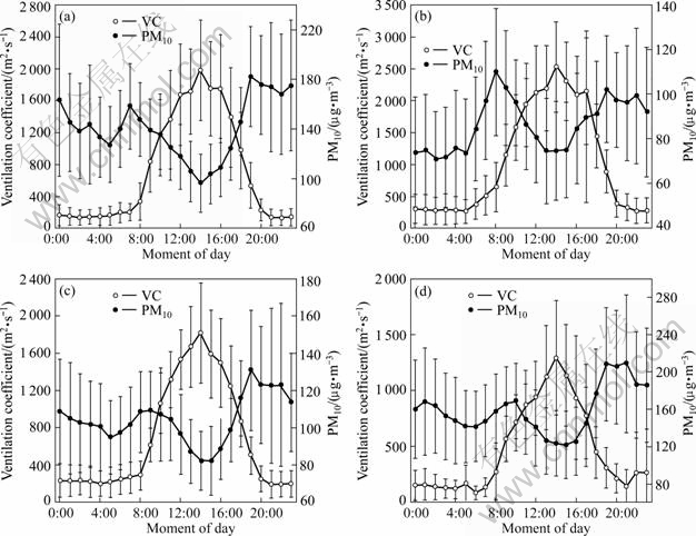
Fig. 4 Correlation between diurnal ventilation coefficient (VC) and PM10 concentration in 2008: (a) Spring; (b) Summer; (c) Autumn; (d) Winter
4 Discussion
Based on the results above, there existed a significant difference of ventilation coefficient between daytime and nighttime. Figure 1 showed that the ventilation coefficient tended to be higher and significantly varied during daytime, while it was relatively lower and constant during nighttime. This may be resulted from the combined effect by the mixing layer height and wind speed. The extreme high values of mixing layer height occurring at noon (14:00) mainly due to the maximum during late night and early morning hours could be explained by the occurrence of ground based inversions which hampered the dispersion [12]. The presence of high-speed wind was common in summer during mid-day, while it was comparatively low in winter months, which corresponded to the average mixing layer height. These observations revealed that the relatively higher ventilation coefficient occurred in daytime, in particular at noon, which was favourable for dispersion of the air pollution. Whereas, the ventilation coefficient seemed low during nighttime, which may hamper the dispersion of air pollutants and thus result in poor air quality. Figure 1 also indicated that both the vertical ventilation (mixing layer height) and the horizontal ventilation (wind speed) were significantly high during noon and afternoon. Both of these two types of ventilation were relatively low during night. The high vertical and horizontal ventilation levels indicated the capacities of dilution and dispersion of air pollutants. MANJU et al [12] estimated the assimilative capacity of Manali on the basis of ventilation coefficient for the four seasons of the year 1998. They found that summer had the highest ventilation coefficient among the various seasons. In their study, the maximum values of the ventilation coefficient were 7 900 m2/s in summer (May) during noon, and the least in winter (January) with value of 2 226 m2/s. In this work, the values in different seasons were averaged by three months, for example, from spring (March, April and May) to winter (December, January and February), and the wind speed was relatively low since it was selected at 10 m above the ground rather than the values at height of atmosphere. So, the ventilation coefficient was relatively lower than the other studies. RAMA et al [20] studied the assimilative capacity based on ventilation coefficient of the Visakhapatnam bowl area in summer and winter of 2002-2003. They demonstrated that the ventilation coefficient was low during early morning and during night, and tended to be the highest during afternoon hours. In their study, the maximum value of ventilation coefficient in summer was 9 781 m2/s and in winter it was 13 924 m2/s at 14:00. By contrast, in terms of the results of this work, the maximum value in summer was greatly larger than that in winter and the values studied were relatively lower than those in the publications mainly due to the different geography and climate in variable terrains.

Fig. 5 Diurnal predicted and observed ventilation coefficient (VC) from January to October in 2010
There are other studies focusing on the variation of the mixing layer height, wind speed and ventilation coefficient in different time segments. Monthly averaged values of morning and afternoon mixing layer height and wind speed were calculated and summarized for seven locations in several climatic regions of the contiguous United States by HOLZWORTH [10]. In his study, the mean afternoon (12:00-16:00) mixing layer height differed by less than 300 m in most months, and mean morning (2:00-6:00) mixing layer height differed by less than 200 m in all months. Comparatively, in this work, the mean mixing layer heights during daytime (8:00-19:00) and nighttime (20:00-7:00) were relatively less than the values in afternoon and morning by HOLZWORTH. In addition, afternoon wind speeds by HOLZWORTH��s study ranged from about 4.5 m/s to 8 m/s and morning speeds varied from 3 m/s to 6.5 m/s. This indicated that the wind speed was greater in the afternoon than that in morning. Compared with his results, nighttime wind speeds in this work ranged from about 1.2 m/s to 1.8 m/s and daytime wind speeds changed from 2 m/s to 3.5 m/s, which interpreted that the wind speed was greater during daytime than nighttime in Changsha. Furthermore, the wind speeds in this work tended to be relatively smaller than the values by other studies probably because the wind speed was selected at the height of 10 m above the ground, which was relatively lower than the heights used in other studies.
The data of mixing layer height and meteorological parameters from January to October in 2010 were adopted using the multi-linear regression model to predict the ventilation coefficient and to test and validate the precision and applicability. Based on Eqs. (2) and (3), the predicted ventilation coefficients were highly close to the observed values. The R2 values of daily observed ventilation coefficient with predicted values were as high as 0.82 (Fig. 5). The high correlation coefficients indicated a relatively good validation of the regression model. Therefore, this model using available meteorological parameters may, to a large extent, accurately predict the real time ventilation coefficient.
5 Conclusions
1) The variation coefficient was significantly variable and high during daytime, while it was relatively invariable and low during nighttime, which indicated that it was reasonable to emit the heavy air pollution during daytime particularly at noon due to the highest ventilation coefficient and capacity for dispersion and dilution of air pollution.
2) The diurnal ventilation coefficient was distinctly negatively correlated with PM10 concentration at the railway station in 2008 in Changsha. The extreme low ventilation coefficient resulted in increasing PM10 pollution during nighttime, which indicated that the ventilation coefficient might play an important role in the variation of PM10 concentration.
3) The multi-linear regression model for ventilation coefficient using some simple meteorological parameters between daytime and nighttime from 2005 to 2009 could be used to accurately calculate and predict the ventilation coefficient of Changsha from January to October in 2010. This model may provide a simple and effective method to forecast the urban ventilation coefficient and thus evaluate the basic variation trend of aerosol pollution.
References
[1] SUN Ye-le, ZHUANG Guo-shun, TANG Ao-han, WANG Ying, AN Zhi-sheng. Chemical characteristics of PM2.5 and PM10 in Haze-Fog episodes in Beijing [J]. Environmental Science and Technology, 2006, 40(10): 3148-3155.
[2] AKPINAR S, HAKAN F O, AKPINAR E K. Evaluation of relationship between meteorological parameters and air pollutant concentrations during winter season in Elaz?g, Turkey [J]. Environmental Monitoring and Assessment, 2007, 146(1/2/3): 211-224.
[3] EMEIS S, SCHAFER K, MUNKEL C. Surface-based remote sensing of the mixing-layer height-A review [J]. Meteorologische Zeitschrift, 2008, 17(5): 621-630.
[4] SCHAFER K, EMERIS S, HOFFMANN H, JAHN C. Influence of mixing layer height upon air pollution in urban and sub-urban areas [J]. Meteorologische Zeitschrift, 2006, 15(6): 647-658.
[5] GHIAUS C, ALLARD F, SANTAMOURIS M, GEORGAKIS C, NICO F. Urban environment influence on natural ventilation potential [J]. Building and Environment, 2006, 41(4): 395-406.
[6] MOTESADDI Z S, KHAJEVANDI M, DAMEZ F D, ARDESTANI M. Determination of air pollution monitoring stations [J]. International Journal of Environmental Research, 2008, 2(3): 313-318.
[7] GOYAL S K, CHALAPATI R C V. Assessment of atmospheric assimilation potential for industrial development in an urban environment: Kochi (India) [J]. Science of the Total Environment, 2007, 376 (1/2/3): 27-39.
[8] MARIA I G, NICOLAS A M. Air pollution potential: Regional study in Argentina [J]. Environmental Management, 2000, 25(4): 375-382.
[9] RIGBY M, TIMMIS R, TOUMI R. Similarities of boundary layer ventilation and particulate matter roses [J]. Atmospheric Environment, 2006, 40(27): 5112-5124.
[10] HOLZWORTH G C. Mixing depths, wind speed and air pollution potential for selected locations in the United States [J]. Journal of Applied Meteorology, 1967, 6(6): 1039-1044.
[11] GOYAL P, RAMA K T. Dispersion of pollutants in convective low wind: A case study of Delhi [J]. Atmospheric Environment, 2002, 36(12): 2071-2079.
[12] MANJU N, BALAKRISHNAN R, MANI N. Assimilative capacity and pollutant dispersion studies for the industrial zone of Manali [J]. Atmospheric Environment, 2002, 36(21): 3461-3471.
[13] AN Xing-qing, ZHU Tong, WANG Zi-fa, LI Cong-ying, WANG Yue-si. A modeling analysis of a heavy air pollution episode occurred in Beijing [J]. Atmospheric Chemistry and Physics, 2007, 7: 3103-3114.
[14] PADMANABHAMURTY B, MANDA, B B. Climatology of inversions, mixing depth and ventilation coefficients at Delhi [J]. Mausam, 1979, 30: 473-478.
[15] KRISHNA TVBPSR, REDDY M K, REDDY R C, SINGH R N. Impact of an industrial complex on the ambient air quality: Case study using a dispersion model [J]. Atmospheric Environment, 2005, 39(29): 5395-5407.
[16] SRIVASTAVA S, LAL S, SUBRAHAMANYAM D B, GUPTA S, VENKATARAMANI S, RAJESH T A. Seasonal variability in mixed layer height and its impact on trace gas distribution over a tropical urban site: Ahmedabad [J]. Atmospheric Research, 2010, 96(1): 79-87.
[17] RIGBY M, TOUMI R. London air pollution climatology: Indirect evidence for urban boundary layer height and wind speed enhancement [J]. Atmospheric Environment, 2005, 42(20): 4932-4947.
[18] GENC D D, YESILYURT C, TUNCEL G. Air pollution forecasting in Ankara, Turkey using air pollution index and its relation to assimilative capacity of the atmosphere [J]. Environmental Monitoring and Assessment, 2010, 166(1-4): 11-27.
[19] GOYAL P, ANAND S, GERA B S. Assimilative capacity and pollutant dispersion studies for Gangtok city [J]. Atmospheric Environment, 2006, 40(9): 1671-1682.
[20] RAMA K, REDDY M K, REDDY R C, SINGH R N. Assimilative capacity and dispersion of pollutants due to industrial sources in Visakhapatnam bowl area [J]. Atmospheric Environment, 2004, 38(39): 6775-6787
(Edited by YANG Bing)
Foundation item: Project(51178466) supported by the National Natural Science Foundation of China; Project(FANEDD200545) supported by Foundation for the Author of National Excellent Doctoral Dissertation of China; Project(2011JQ006) supported by Fundamental Research Funds of the Central Universities of China
Received date: 2011-07-26; Accepted date: 2011-11-14
Corresponding author: DENG Qi-hong, Professor, PhD; Tel: +86-731-88877175; E-mail: qhdeng@csu.edu.cn
Abstract: The temporal variation of ventilation coefficient was estimated and a simple model for the prediction of urban ventilation coefficient in Changsha was developed. Firstly, Pearson correlation analysis was used to investigate the relationship between meteorological parameters and mixing layer height during 2005-2009 in Changsha, China. Secondly, the multi-linear regression model between daytime and nighttime was adopted to predict the temporal ventilation coefficient. Thirdly, the validation of the model between the predicted and observed ventilation coefficient in 2010 was conducted. The results showed that ventilation coefficient significantly varied and remained high during daytime, while it stayed relatively constant and low during nighttime. In addition, the diurnal ventilation coefficient was distinctly negatively correlated with PM10 (particle with the diameter less than 10 ��m) concentration in Changsha, China. The predicted ventilation coefficient agreed well with the observed values based on the multi-linear regression models during daytime and nighttime. The urban temporal ventilation coefficient could be accurately predicted by some simple meteorological parameters during daytime and nighttime. The ventilation coefficient played an important role in the PM10 concentration level.
