J. Cent. South Univ. (2016) 23: 2048-2062
DOI: 10.1007/s11771-016-3261-3

Multi-species particle swarms optimization based on orthogonal learning and its application for optimal design of a butterfly-shaped patch antenna
SUN Li-ling(������)1, 2, 3, HU Jing-tao(������)1, HU Kun-yuan(����Ԫ)1,
HE Mao-wei(��ïΰ)1, 2, 3, CHEN Han-ning (�����)3
1. Department of Information Service & Intelligent Control, Shenyang Institute of Automation,Chinese Academy of Sciences, Shenyang 110016, China;
2. University of Chinese Academy of Sciences, Beijing 100039, China;
3. School of Computer Science and Software, Tianjin Polytechnic University, Tianjin 300387, China
 Central South University Press and Springer-Verlag Berlin Heidelberg 2016
Abstract:
A new multi-species particle swarm optimization with a two-level hierarchical topology and the orthogonal learning strategy (OMSPSO) is proposed, which enhances the global search ability of particles and increases their convergence rates. The numerical results on 10 benchmark functions demonstrated the effectiveness of our proposed algorithm. Then, the proposed algorithm is presented to design a butterfly-shaped microstrip patch antenna. Combined with the HFSS solver, a butterfly-shaped patch antenna with a bandwidth of about 40.1% is designed by using the proposed OMSPSO. The return loss of the butterfly-shaped antenna is greater than 10 dB between 4.15 and 6.36 GHz. The antenna can serve simultaneously for the high-speed wireless computer networks (5.15�C5.35 GHz) and the RFID systems (5.8 GHz).
Key words:
1 Introduction
Patch antennas are widely used in wireless communication systems because of their advantages, such as low profile, light weight, and ease in fabrication. Many efforts have been done on the parametric study of various patch antennas [1-4]. However, most of these studies are dependent on the antenna under investigation. Therefore, in most patch antenna designs, a trial-and-error process is necessary. Clearly, this process is time consuming and will not necessarily give the optimum parameters. Thus, a powerful optimization technique is needed, which will enable the antenna designer to design a specific antenna that meets specific requirements [5].
As the geometrical shapes and spatial structures of patch antennas become more complicated and the number of the optimization parameters becomes larger, the classical derivative-based optimization techniques are prone to getting trapped in local optima and strongly sensitive to initialization. The heuristic algorithms based on the principles of biological evolution have been successfully applied in optimization and design of antennas, due to their strong capability of global search. For example, TELZHENSKY and LEVIATHAN [6] used the genetic algorithm (GA) to optimize UWB antenna for specified input signal forms; ANURADHA et al [7] designed and optimized a new fractal tree antenna using particle swarm optimization (PSO) algorithm; DACUNA and POUS [8] applied a hybrid approach involving bacterial foraging algorithm (BFA) to design a bow-tie antenna for 2.45 GHz radio frequency identification (RFID) readers.
In this paper, inspired by the mutualism phenomenon, a new multi-species particle swarm optimization with a two-level hierarchical topology and the orthogonal learning strategy (OMSPSO) is proposed to optimize antenna. The proposed algorithm extends the single population PSO to the interacting multi-swarms model by constructing hierarchical information networks. In our proposed multi-species particle swarm optimizer, the position of each individual updates according to not only its personal best position and the global best position of its sub-population but also the different global best positions of other sub-populations. When tested against benchmark functions, the OMSPSO markedly outperforms the classical PSO, CPSO, GA, and DE algorithms in terms of accuracy, robustness and convergence speed.
The OMSPSO (implemented in MATLAB) is used along with the high frequency structure simulator (HFSS) software, which is an electromagnetic simulator, to design a butterfly-shaped microstrip patch antenna with air gap for the requirement of RFID systems (5.8 GHz) and high-speed wireless computer networks (5.15�C5.35 GHz). The patch geometry is cut into a butterfly shape which offers satisfactory performances by only adjusting the diameter of the radiant arms and the position of the circular slots. In addition, the frequency band and the return loss can be adjusted by these parameters independently. The numerical simulations are performed using HFSS software. With optimization of the OMSPSO, a wideband butterfly-shaped antenna, which has 40.1% bandwidth and a return loss greater than 10 dB in the frequency band between 4.15-6.36 GHz, has been designed. These characteristics are very desirable for RFID systems and high-speed wireless computer networks.
2 Explanation of algorithm
2.1 Canonical particle swarm optimization
Particle swarm optimization (PSO) is an evolutionary computation (EC) algorithm paradigm that emulates the swarm behaviors of birds flocking [9]. It is a population-based search algorithm that exploits a population of individuals to probe promising regions of the search space. In this context, the population is called a swarm, and the individuals are called particles. Each particle moves with an adaptable velocity within the search space and retains in its memory the best position it ever encountered. The standard version of PSO is briefly described here [10-11].
Let s be the swarm size, d be the particle dimension space, and each particle of the swarm have a current position vector Xi, a current velocity vector Vi, and an individual best position vector Pi found by the particle itself so far. The swarm also has the global best position vector Pg found by any particle during all prior iterations in the search space. Assuming that the function f(X) is to be minimized, and describing the following notations in tth iteration, the definitions are as follows:

 (1)
(1)
where each dimension of a particle is updated using the following equations:

 (2)
(2)
 (3)
(3)
In Eq. (2), c1 and c2 denote constant coefficients and r1 and r2 are elements from random sequences in the range of (0, 1).
The inertia weight w plays the role in balancing the global and local searches. It can be a positive constant (e.g., 0.9) or even a positive linear or nonlinear function of time [10-11]. Although sometimes proper fine-tuning of the parameters c1 and c2 leads to an improved performance, an extended study of the cognitive and social parameters was proposed in Ref. [12], and c1 = c2 = 2 were proposed as default values.
2.2 Multi-species coevolution model for optimization
In this section, the model for the coevolution of multi-species is described and the formulation of the multi-species particle swarm optimization is proposed.
The notion of multi-species has been introduced in some variant version of the PSO algorithm. A multi-species PSO (MS-PSO) was proposed by CHOW and TSUI [13]. In early research, a multi-swarm cooperative particle swarm optimizer (MCPSO) was described in Ref. [14]. In MCPSO, the population consists of one master swarm and several slave swarms. The slave swarms execute the canonical PSO algorithm or its variants independently and the particles in the master swarm enhance themselves based on their own knowledge and also the knowledge of the particles in the slave swarms. Due to the disadvantage of no information sharing among slave swarms, the master guided by the slave swarms may suffer premature convergence.
2.2.1 Proposed multi-species optimizer
Inspired by the mutualism phenomenon, we extend the single population PSO to the interacting multi-swarms model by constructing hierarchical information networks. In our proposed multi-species particle swarm optimizer, the position of each individual updates according to not only its personal best position and the best position of its sub-population but also the different best positions of other sub-populations. Therefore, each individual moving through the solution space should be influenced by three attractors:
1) Its own previous best position;
2) Best position of its neighbors from its own species;
3) Best position of its neighbor species.
In mathematical terms, the particle��s fly velocity Eq. (2) and position update Eq. (3) are thus changed as

 (4)
(4)
 (5)
(5)
where the superscript k denotes the kth species of the total M species;  represents the position of the ith particle of the kth species;
 is the personal best position found so far by
 is the best position found so far by this particle��s neighbors within the kth species;
  is the best position found so far by the other neighborhood species (the superscript �� is the index of the swarm which the best position belongs to); c1, c2 and c3 denote constant coefficients and r1, r2 and r3 are elements from random sequences in the range of (0, 1).
The second term  of Eq. (4) is associated with the cognition component since it takes into account the individual��s own experiences; the third term
  represents the social interaction within the kth swarm; the fourth term
  takes into account the symbiotic coevolution between dissimilar species.
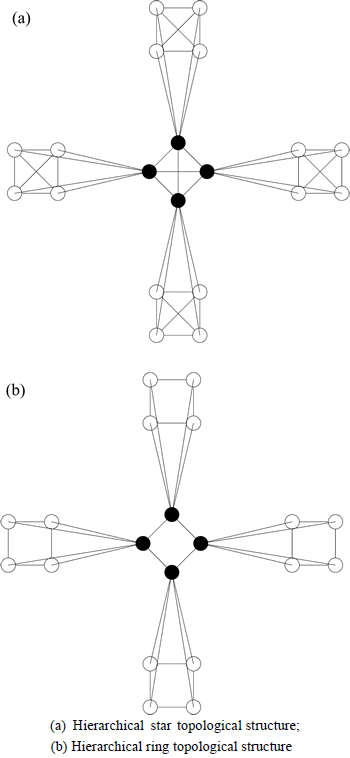
Fig. 1 Two-level interaction topologies:
2.2.2 Hierarchical interaction topology
To implement cooperation, two-level interaction topologies (corresponding to the individual level and the swarm level) are constructed, as shown in Fig.1. The information communication simultaneously occurs in and between these two levels. In the first topology (namely the 2-level star topology, shown in Fig. 1(a)), each individual is influenced by the performance of its own species and all the other species in the ecosystem. In the second topology (namely the 2-level ring topology, shown in Fig. 1(b)), each individual is influenced only by n closest neighbours from its own species and other n species from the ecosystem.
2.3 Orthogonal experimental design
2.3.1 Traditional PSO learning mechanism
In the traditional PSO, each particle updates its flying velocity and position according to its personal best position and the global best position. The concept is simple and appealing, but this learning strategy can cause the ��two steps forward, one step back�� phenomenon and the ��oscillation�� phenomenon [15].
A prominent phenomenon of the traditional learning mechanism, which inevitably happens in the process of searching the global best position, is the ��two steps forward, one step back�� phenomenon [16]. For example, consider a three-dimension vector X=(x1, x2, x3), and the fitness function f (X) = (x1-20)2 + (x2-20)2 + (x3-20)2, whose optimal position is [20, 20, 20]. Suppose that the current position is X(t) = [5, 20, 5] with the fitness value of 450 and the global best position searched by the population so far is Pg = [17, 2, 17] with fitness value of 342. According to Eqs. (2) and (3), the new position is X(t+1) = [15, -5, 15], whose fitness value is 275 better than the global best position. It means that the global best position Pg will be update now. However, the second component of the vector has changed from the correct value of 20 to the rather poor value of 5; thus the valuable information has been lost unknowingly. If we can discover the good components of the vector, the particle may fly toward to the better position [17, 20, 17]. Another ��oscillation�� phenomenon is likely to be caused by liner summation of the personal influence and the global influence. For the clearness and easiness of understanding, the inertia weight term of Eq. (2) is removed and the random coefficients are set as constants. The final expression of velocity equation is as follows:
 (6)
(6)
In Eq. (6), we consider the following case for a maximization problem where the current particle Xi is between its personal best position Pi and the global best position Pg, as shown in Fig. 2. At first, the distance between Pg and Xi may be farther than the one between Pi and Xi, as in Fig. 2(a), and then Xi will move toward Pg because of its larger pull. However, as moving toward Pg, the distance between Pi and Xi will increase, as shown in Fig. 2(b). In this case, the particle will move toward Pi instead. The oscillation would thus occur and the particle will be puzzled in deciding where to stay [15]. This oscillation phenomenon causes inefficiency to the search ability of the algorithm and delays convergence.
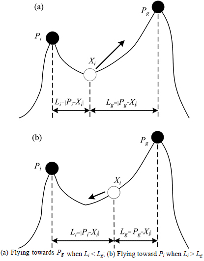
Fig. 2 Oscillation phenomenon in PSO:
2.3.2 Orthogonal learning strategy
Concepts of OED: We use a simple example to illustrate how to use the OED. More detailed information can be found from [17-20]. This example arises from chemical experiments. The conversion ratio of a chemical experiment depends on three variables: temperature (A), time (B), and alkali (C). These three quantities are called the factors of the experiment. Each factor has three possible values listed in Table 1 [17], and we say that each factor has three levels.
To find the best combination of levels for a maximum conversion ratio, we can do one experiment for every combination and then select the best one. In the aforementioned example, there are, in total, 33 = 27 combinations of experimental designs. In general, when there are N factors and Q levels per factor, there are QN combinations. When N and Q are large, it is not possible or efficient to test all the combinations in the case. With the help of OED, it is efficient to obtain or predict the best combination by testing only few representative experimental cases.
1) Orthogonal array (OA): The OED method works on a predefined table called an orthogonal array, represented as LM(QN) with N factors and Q levels per factor. L denotes the orthogonal array and M is thenumber of combinations of test cases. The L9(34) OA given is shown in Eq. (7), which has four factors, three levels per factor and nine combinations of levels. The first three columns in the first row is [1, 1, 1], meaning that in this experiment, the first factor (temperature), the second factor (time), and the third factor (alkali) are all designed to the first level, that is, 80 ��C, 90 min, and 5% as given in Table I.
 (7)
(7)
2) Factor analysis: The factor analysis (FA), which based on the experimental results of all the M cases of OA, can evaluate the best combination of levels on the experimental results. The results of FA are listed in Table 2 and the analysis process is described as follows:
Table 1 Orthogonal array of the orthogonal experimental design
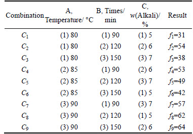
Let fm denote the experimental result of the mth (m = 1, 2, . . ., M) and Snq denote the effect of the qth (q = 1, . . . , Q) level in the nth (n = A, B, C) factor. The calculation of Snq is to add up all the fm in which the level is q in the nth factor, and then divide the total count of Zmnq, as follows:
 (8)
(8)
where Zmnq is 1 if the mth experimental test is with the qth level of the nth factor, otherwise, Zmnq is 0.
In this way, the effect of each level on each factor can be calculated and compared, as listed in Table 2.
Table 2 Deciding best combination levels of chemical experimental factors using an OED method

For example, when we calculate the effect of level 1 on factor A, denoted by element A1, the experimental results of C1, C2, and C3 are summed up for Eq. (8) because only these combinations are involved in level 1 of factor A. Then, the sum divides the combination number (3 in this case) to yield Snq (SA1 in this case). After all the Snq��s are calculated, the best level of each factor can be determined by selecting the level of each factor that provides the highest quality Snq. As the example shown in Table 2 is a maximization problem, the larger the Snq, the better the qth level on factor n is. Otherwise, vice versa. Thus, the best combination of (A3, B2, C2) can be obtained.
3) Orthogonal learning strategy:
With the help of OED method, the traditional PSO can be modified with orthogonal learning (OL) strategy. The new position vector of an individual is determined by its personal best position vector  the best position of its neighbors from its own species
  and the best position of its neighbor species
  to form a better guidance vector
  The particle��s fly velocity Eq. (2) is thus changed as
 (9)
(9)
where c is fixed as 2 and rd is a random value in the range of (0, 1).
Owning to the efficient learning strategy of OED, the particle with a guidance vector  has a higher probability of moving to a better position. Especially, for solving high-dimensional problems, the orthogonal learning strategy may have a better performance on local search.
2.4 Algorithmic framework
In this work, we intend to use the orthogonal experimental design method to improve the search ability of the multi-species particle swarm optimization with two-level hierarchical topology, especially the local search ability for the high-dimensional problems. The flowchart of OMSPSO is shown in Fig. 3.
2.5 Experimental study
Here, we discuss the computational results, and analyze the performance of our algorithm against other state-of-the-art algorithms.
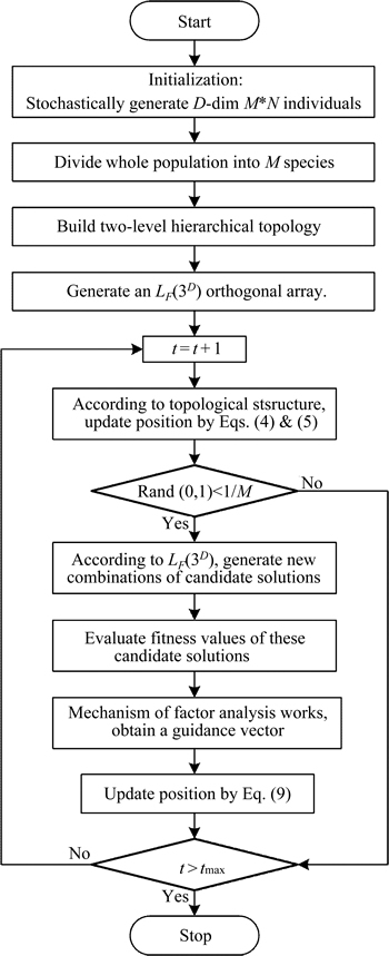
Fig. 3 Flowchart of OMSPSO
2.5.1 Experimental settings
The orthogonal learning based multi-species particle swarms optimization (OMSPSO) were executed with for state-of-the-art EA and SI algorithms for comparisons: canonical particle swarm optimization [13], cooperative particle swarm optimization (CPSO) [16], differential evolution (DE) [19], and standard genetic algorithm (GA) [20].
In all experiments in this section, the values of the common parameters used in each algorithm such as population size and total generation number are chosen to be the same. Population size is set as 100 and the maximum evaluation number is set as 100000. For the continuous testing functions used in this work, the dimensions are all set as 10D, 30D.
All the control parameters for the EA and SI algorithms are set to be default in their original literatures: The split factor for CPSO is equal to the dimensions [16]. For canonical PSO and CPSO, the learning rates c1 and c2 are both set as 2.0 and the inertia weight decreases from 0.9 to 0.4. For GA, the crossover rate of 0.8 and the mutation rate of 0.01 are adopted [20]. For our proposed algorithm, the whole population is divided into 10 sub-populations (also called 10 species). Each species includes 10 individuals. The learning rates c1, c2 and c3 in Eq. (4) are all set as 1.3667 and the learning rate c in Eq. (9) is set as 2.0.
In this section, we will test the performance of OMSPSO with the ring topology (upper level and lower level both with ring topologies, namely OMSPSO-R) and OMSPSO with the star topology (upper level and lower level both with star topologies, namely OMSPSO-S).
2.5.2 Test and benchmark problems
According to the no free lunch theorem, ����for any algorithm, any elevated performance over one class of problems is exactly paid for in performance over another class���� [21]. To fully evaluate the performance of the OMSPSO-R and OMSPSO-S without a biased conclusion towards some chosen problems, a set of ten benchmark function is employed. The formulas of these functions are presented below.
1) Rosenbrock function,
 (10)
(10)
2) Quadric function,
 (11)
(11)
3) Sum of different powers,
 (12)
(12)
4) Axis parallel hyper-ellipsoid function,
 (13)
(13)
5) Sphere function,
 (14)
(14)
6) Ackley��s function,

 (15)
(15)
7) Griewank function,
 (16)
(16)
8) Michalewicz function,
 (17)
(17)
9) Rastrigrin��s function,
 (18)
(18)
10) Schewfel function,
 (19)
(19)
These ten benchmark functions can be grouped as unimodal continuous functions f1-f5 and multimodal continuous functions f6-f10.
2.5.3 Result and statistical analysis
In this experiment, we compared two variant versions of OMSPSO algorithm with the canonical PSO algorithm, CPSO algorithm, DE algorithm, and GA algorithm. Table 3 shows the basic statistical results (i.e. the mean and standard deviations of the function values found in 30 runs) of the 10D benchmark test functions f1-f10 introduced above. From the table, obviously, the canonical PSO and GA algorithms demonstrate the worse performance than other four algorithms. The PSO��s variants outperform the canonical PSO algorithm, due to the OMSPSO-R, OMSPSO-S and CPSO have their own strategies to overcome the ��two steps forward, one step back�� phenomenon. For the low-dimensional (10D) unimodal functions f1-f5, the DE algorithm is comparatively good among these algorithms. The results of the OMSPSO algorithms are also competitive if not better than the results of other algorithms and it is able to find the minimum to functions f1 and f3. The two variants of OMSPSO algorithms have nearly the same results for low-dimensional problems. For the low-dimensional (10D) multimodal functions f6-f10, intuitively, the OMSPSO-R algorithm has rather smaller mean values and standard deviations than other algorithms for f8, f9, and f10 test functions. Meanwhile, for test functions f6 and f7, the results of OMSPSO-R and OMSPSO-S algorithms are still considerably good although not the best ones. This is attributed to that the topological structure of the upper level and lower level both with rings can well keep the individual diversity during the search process and avoid to get trapped into the local optimal, which is important for solving the multimodal problems.
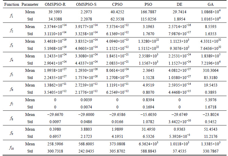
Table 4 presents the basic statistical results of the 30D benchmark test functions f1-f10. The mean and standard deviations of the function values are found in 30 runs for each algorithm on each function. With the increase of the dimensions, the convergence rate becomes slow and the difference among the statistical results becomes larger. For the high-dimensional unimodal problems f1-f5, the performance of OMSPSO algorithms gradually turns better, which is due to the orthogonal experimental design method displays a higher efficiency for predicting the best combinations of higher levels (higher dimensions) with many factors. From Table 4, the OMSPSO-R algorithm is suitable for solving f3 and f4 problems and the OMSPSO-S algorithm has the smallest mean values and standard deviations for f1 and f5 test functions. For test function f2, compared with the canonical PSO algorithm, the performance of the OMSPSO algorithms has an extremely improvement. For solving the high- dimensional multimodal problems f6-f10, the OMSPSO-R has an outstanding performance. This is because that, compared with the good performance of CPSO algorithm for only solving the ��two steps forward, one step back�� phenomenon, the OMSPSO-R algorithm simultaneously overcomes both ��two steps forward, one step back�� and ��oscillation�� phenomena. With the two-level hierarchical ring topology, the OMSPSO-R algorithm can well avoid premature convergence to local optimal in the process of solving the high-dimensional multimodal problems.
Table 3 Performance of all algorithms on 10D test functions f1-f10
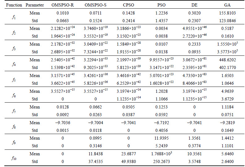
Table 4 Performance of all algorithms on 30D test functions f1-f10.
The convergence curves of the OMPSO algorithms and other EAs against test functions f1-f10 in 10D and 30D are shown in Figs. 4 and 5. It can be observed that, with the increase of the dimensions, the convergence rate of OMSPSO becomes faster. Predictably, with a further increase of the dimensions of the test functions, the OMSPSO-R algorithm will have an overwhelming superiority in solving the high-dimensional problems.
3 Antenna optimization using OMSPSO
Nowadays, high-speed wireless communication networks have attracted the attention of researchers, especially in the 5-6 GHz band. This band can cover the frequencies of the high-speed wireless computer networks (e.g., IEEE 802.11a) [22] and the RFID UHF band in North America [23]. Such networks have the ability to provide high-speed connectivity (>50 Mb/s) among notebook computers, PCs, personal organizers, and other wireless digital appliances. To operate in complex environments, such as buildings, factories, hospitals, railway stations, and airports, an antenna has to own a wider operating band.
In this section, a novel single-patch wideband microstrip antenna with air gap for the requirement of RFID systems (5.8 GHz) and high-speed wireless computer networks (5 GHz) is present. The proposed antenna, cut into a butterfly shape, is designed to cover these frequency bands. With the help of the proposed OMSPSO (implemented in MATLAB) and electromagnetic simulation (implemented through VB script of HFSS), the parameters of the butterfly-shaped antenna are optimized to obtain wider band.
3.1 Antenna geometry
The geometry of the antenna which is cut into a butterfly shape is shown in Fig. 6. Through adjusting the diameter of the radiant arms and the position of the circular slots the antenna can offer satisfactory performances. In addition, the frequency band and the return loss can be adjusted by these parameters independently. So, the OMSPSO-R is applied to optimization of the parameters of the antenna. As shown in Fig. 6, the proposed antenna consists of a butterfly- shaped metallic patch suspended which is composed of two symmetric small loops and 3/4 loops linked together, by means of a 5.5 mm thick air gap (��r=1), over an 80��80mm2 ground plane. The patch is centered at the middle of the ground plane. The antenna is fed with a coaxial probe at position Px from the geometric center of the microstrip line. The feed point is welded at the 50 �� SMA coaxial connector. Moreover, the width W and the length L of the microstrip line exciting the antenna, the inner radius Rin1, Rin2 and outer radius Rout1, Rout2 of both metallic loops forming the radiating arms have to be optimized. This gives a total of seven parameters to be determined by the optimization algorithms to find the best configuration for the butterfly-shaped patch antenna targeting widen the operation band without adding other structures. The parameters required to be optimized are listed in Table 5.
3.2 Optimal antenna designformulation
For the optimization of the butterfly-shaped geometry, one objective and several constrains are set up which define the performance of the antenna.
The optimization goals are incorporated into the fitness function defined in Eq. (20), where the minimization of the fitness produces a wider band.
 (20)
(20)
where NS11 is the number of the frequency points, the reflection coefficients S11 of which are less than -10 dB; f denotes frequency point. Here, we choose 351 frequency points between 4 GHz and 7.5 GHz.
This optimization constitutes an N=7 dimensional problem, where all dimensions are shown in Fig. 6 and the corresponding ranges are listed in Table 6. To avoid the overlap problem in HFSS simulations, the following conditions Eqs. (21) to (28) must be held as additional geometrical restrictions:
 (21)
(21)
 (22)
(22)
 (23)
(23)
 (24)
(24)
 (25)
(25)
 (26)
(26)
 (27)
(27)
 (28)
(28)
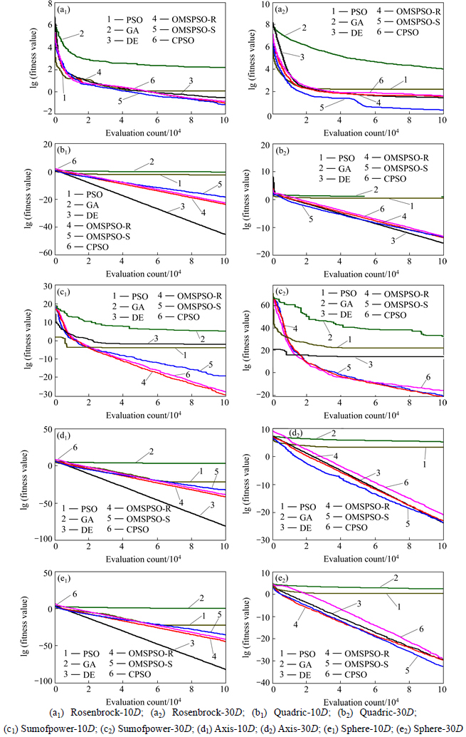
Fig. 4 Convergence curves of PSO, GA, DE, CPSO, OMSPSO-R and OMSPSO-S against test functions f1-f5 in low dimension 10D and high dimension 30D, respectively:
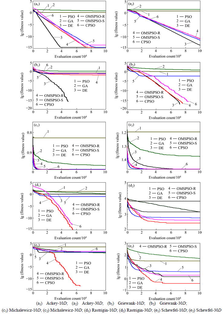
Fig. 5 Convergence curves of PSO, GA, DE, CPSO, OMSPSO-R and OMSPSO-S against test functions f6-f10 in low dimension 10D and high dimension 30D, respectively:
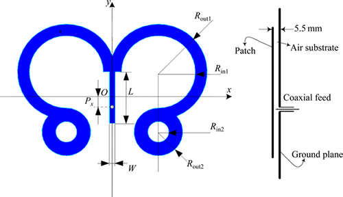
Fig. 6 Schematic representation of proposed butterfly-shaped patch antenna
Table 5 Parameters of butterfly-shaped antenna to be optimized
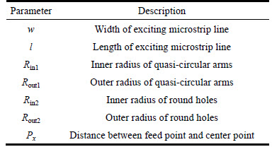
Table 6 Minimum and maximum allowed limits for each of optimization parameters (Unit: mm)

3.3 Constraints handle
As mentioned above, the design and optimization of the butterfly-shaped patch antenna is a constrained optimization problem. To solve constrains, this work uses a modified way to handle constraints which is introduced by ALI [24]. According to the DEB��s method [25] which requires any individual to comply with the constraints, the modified method considers both the fitness value and the constraints. Three new rules are as follows:
1) The trial vector is feasible and the target vector is not.
2) The trial vector and target vector are both feasible, but the trial vector has smaller than or equal fitness value than the corresponding target vector.
3) The trial vector and target vector are both infeasible, but the trial vector has smaller than or equal overall constraint violation than the corresponding target vector.
The above selection procedure allows the trial vector to be entered in the new population if it has the same amount of constraint violation or objective function value as the target vector. Therefore, this simple modification can help the algorithm to spread out and pass through the search space, so the algorithm can escape from stagnation.
3.4 Implementation of OMSPSO algorithm for antenna design
To apply the OMSPSO to optimize and design the butterfly-shaped patch antenna, the following steps should be taken and repeated.
Step 1: Initialization
1) Antenna parameters initialization
In the proposed antenna, there are seven adjustable parameters to be optimized, which have been listed in Table 5. These parameters are combined into a vector with N=7 dimensions, x=(x1, x2, x3, x4, x5, x6, x7)=(W, L, Rout1, Rin1, Rout2, Rin2, Px). And the boundary limits of each dimension is defined in Table 8. Every dimension is generated randomly as follows:
 (29)
(29)
where  and
and  are the maximum and minimum boundary limits listed in Table 8, respectively; random denotes a uniformly distributed number between [0, 1].
If the dimension values of one vector can��t meet the constraints Eqs. (21) to (26), then this vector will be re-generated until it meets all these constraints.
2) OMSPSO initialization
The specific parameter of the proposed OMSPSO are set as the same as them in section 2.5.1. The optimizers are applied for only one trial of 15000 evaluations. Here, a maximum stagnation times of constraints handling is set as 30.
Step 2: Optimization procedure
1) Fitness calculation
In calculating the fitness value, the simulation results (a series of the reflection coefficients S11) may not meet the design requirements listed in the Eqs. (27) and (28). In this situation, the fitness value is set as 2.
During the optimization procedure, the simulation results may have multiple bandwidths (S11��-10 dB) and meets the design requirements. In this situation, the fitness value is calculated according to the maximum bandwidth.
2) constrains handle in optimization of butterfly- shaped patch antenna.
During optimization process, if an individual continually places beyond the constraints and its stagnation times of constraint handling achieve the limits (30 times), its unmatched dimensions will be fixed near the constraint limits as following:


where  and
and  are the maximum and minimum of the constraint boundaries of the ith dimension which are calculated according to Eqs. (21) to (26).
And Eqs. (21) to (26) can be synthesized as follows:

 (30)
(30)
Then, the constraint condition of each dimension is simplified as follows:
 (31)
(31)
 (32)
(32)
 (33)
(33)
 (34)
(34)
 (35)
(35)
 (36)
(36)
 (37)
(37)
If the number of unmatched dimensions is more than 1, the adjustment operation needs to run many times until no unmatched dimension exists.
Step 3: Termination condition
If the current iteration number achieves the preordained maximum iteration number, the optimization is stopped; otherwise, go to Step 2.
Table 7 Dimensions of final optimized butterfly-shaped patch antenna (Unit: mm)


Fig. 7 Convergence curves of OMSPSO, GA, PSO for optimizing parameters of butterfly-shaped patch antenna
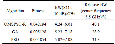
Table 8 Results of optimizing butterfly-shaped patch antenna
4 Simulation and measurement results
4.1 Antenna optimization
According to the analysis in Section 2, the proposed OMSPSO has a good performance in solving continuous optimization problems. Here, a comparison among the OMSPSO, genetic algorithm (GA) and particle swarm optimization (PSO) algorithm for optimizing the parameters of the above butterfly-shaped patch antenna is given, which can verify the OMSPSO is also very suitable for optimization of antennas.
The specific parameters of the OMSPSO-R, GA and PSO are listed in Section 2.2.2. The optimizers are applied for only one trial of 15000 evaluations and the population size is 30.
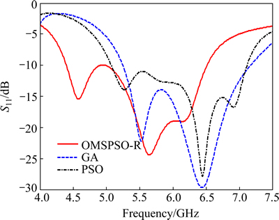
Fig. 8 Return loss of butterfly-shaped patch antenna optimized by OMSPSO-R, GA and PSO algorithms
The parameters of the final optimized designs are provided in Table 7. And the convergence curves are shown in Fig. 7. From this figure, it is obvious that OMSPSO outperforms GA and PSO for optimization of this antenna in terms of accuracy and convergence speed.
The reflection coefficients S11 of the optimized butterfly-shaped patch antenna are illustrated in Fig. 8. And the detailed characteristics of the butterfly-shaped patch antenna optimized by three algorithms are listed in Table 7. From the results of the fitness function, the antenna design optimized by OMSPSO-R is smaller than the other two because OMSPSO-R has faster convergent speed and more excellent global optimization ability than GA and PSO. As revealed in Table 8, the antenna optimized by OMSPSO-R has largest bandwidth and relative bandwidth among these three antennas, which sufficiently meets the design requirement (bandwidth of 5-6 GHz).
As mentioned above, the butterfly-shaped patch antenna with the optimized parameters using the OMSPSO-R has a better performance. Therefore, in the rest of this section, the numerical and experimental results of this antenna are provided and discussed in detail.
4.2 Current distribution
Figure 9 depicts the surface current distribution excited on the butterfly-shaped antenna at the frequencies of 4.4 GHz, 5.5 GHz and 6.2 GHz, respectively. In particular, from Fig. 9(a), it appears that at 4.4 GHz, the current distribution concentrates on the radiating arms close to the exciting microstrip line. This current behavior is due to the increment of the current path caused by the removal of the inner circles of the 3/4 loops forming the radiating arms, while at 5.5 GHz, a typical ��/2 resonant antenna current distribution is excited in the radiating arms (Fig. 9(b)). Finally, at 6.6 GHz all the metallic surfaces of the antenna are affected by the surface current as it appears from Fig. 9(c).
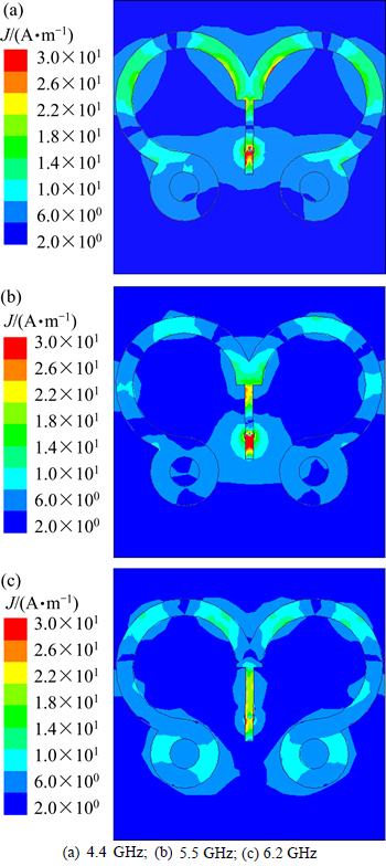
Fig. 9 Current distribution of proposed antenna at different frequencies (Simulation in HFSS software):
4.3 Measurement results
The photograph of the optimized antenna prototype is shown in Fig. 10. The butterfly-shaped patch and the extended ground plane have been manufactured using conductive copper tape with 1mm thickness. The simulated and measured reflection coefficients of the antenna are shown in Fig. 11. The measurements are performed using an Agilent E5071C network analyzer. Considering a bandwidth of -10 dB, the experimental value of the relative bandwidth to the center frequency (5.5 GHz) is 40.1%, while the corresponding value obtained by numerical simulation is of about 41.7%. A good agreement between the simulated and experimental results is observed. It addition, it can be noticed that the antenna has sufficient bandwidth to cover the requirement of the RFID systems and the wireless computer networks.
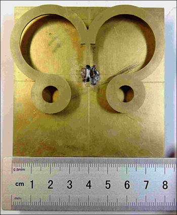
Fig. 10 Photograph of proposed antenna
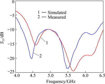
Fig. 11 Measured and simulated frequency behavior of magnitude of reflection coefficient
4.4 Antenna radiation pattern
The tridimensional radiation pattern of the proposed antenna, computed at 5.8 GHz, is shown in Fig. 12. The antenna radiates nearly unidirectional from the top side of the ground plane. Fig. 13 shows the simulated antenna gain for frequencies across the operating bands. The range of the antenna gain is 4.0-8.6 dB. In particular, at 5.8 GHz the corresponding gain is 8.3dB, while at 5.0 GHz is 4.4 dB.
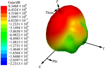
Fig. 12 3-D gain pattern at 5.8 GHz
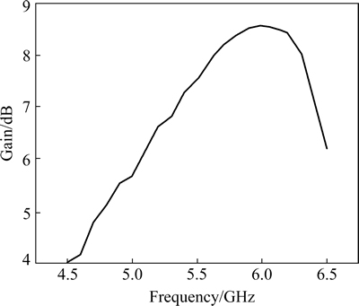
Fig. 13 Computed antenna gain versus frequency
5 Conclusions
We have presented a novel multi-species PSO algorithm with a two-level hierarchical topology and orthogonal learning strategy, named OMSPSO. The two-level hierarchical topology enriches the individual diversity and the orthogonal experimental design method improves the performance of local search, which can excellently overcome the ��oscillation�� phenomenon and ��two steps forward, one step back�� phenomenon in the high-dimensional problems. To identify the effectiveness of the proposed algorithm, the OMSPSO was compared with previously proposed GA, PSO, CPSO and DE. In addition, the algorithm is applied to optimize a patch antenna. The measurements of the designed antenna meet our requirement for the high-speed wireless communication network and the radio frequency identification system. And we believe OMSPSO has a great application potential in a variety of complex real-world problems.
References
[1] KIOURTI A, NIKITA K S. A review of implantable patch antennas for biomedical telemetry: Challenges and solutions [J]. IEEE Antennas and Propagation Magazine, 2012, 54(3): 210-228.
[2] WANG Zhong-bao, FANG Shao-jun, FU Shi-qiang, JIA Shou-li. Single-fed broadband circularly polarized stacked patch antenna with horizontally meandered strip for universal UHF RFID applications [J]. IEEE Transactions on Microwave Theory and Techniques, 2011, 59(4): 1066-1073.
[3] DONG Yuan-dan, TOYAO H, ITOH T. Compact circularly-polarized patch antenna loaded with metamaterial structures [J]. IEEE Transactions on Antennas and Propagation, 2011, 59(11): 4329�C 4333.
[4] ABUTARBOUSH H F, NILAVALAN R, CHEUNG S W, NASR K M, PETER T, BUDIMIR D, AL-RAWESHIDY H. A reconfigurable wideband and multiband antenna using dual-patch elements for compact wireless devices [J]. IEEE Transactions on Antennas and Propagation, 2012, 60(1): 36�C43.
[5] NAKAMURA T, FUKUSAKO T. Broadband design of circularly polarized microstrip patch antenna using artificial ground structure with rectangular unit cells [J]. IEEE Transactions on Antennas and Propagation, 2011, 59(6): 2103�C2110.
[6] TELZHENSKY N, LEVIATAN Y. Novel method of UWB antenna optimization for specified input signal forms by means of genetic algorithm [J]. IEEE Transactions on Antennas and Propagation, 2006, 54(8): 2216�C2225.
[7] ANURADHA A, PATNAIK A, SINHA S N. Design of custom-made fractal multi-band antennas using ANN-PSO [J]. IEEE Antennas and Propagation Magazine, 2011, 53(4): 94�C101.
[8] DACUNA J, POUS R. Low-profile patch antenna for RF identification applications [J]. IEEE Transactions on Microwave Theory and Techniques, 2009, 57(5): 1406�C1410.
[9] KENNEDY J, EBERHART R C. Particle swarm optimization [C]// Proceedings of IEEE International Conference on Neural Networks, Perth, Australia: IEEE, 1995: 1942�C1948.
[10] SHI Y, EBERHART R C. Parameter selection in particle swarm optimization [C]// Proceedings of Evolutionary Programming. Perth, Australia: PEP, 1998: 591-600.
[11] SHI T, EBERHART R C. A modified particle swarm optimizer [C]// Proceedings of IEEE International Conference on Evolutionary Computation. Berlin, Germany: IEEE, 1998: 69-73.
[12] KENNEDY J. The particle swarm: social adaptation of knowledge [C]// Proceedings of IEEE International Conference on Evolutionary Computation. Berlin, Germany: IEEE, 1998: 303-308.
[13] CHOW C K, TSUI H T, Autonomous agent response learning by a multi-species particle swarm optimization [C]// Proceeding of Congress on Evolutionary Computation. Portland, Oregon, USA: PCEC, 2008: 778-78.
[14] NIU Ben, ZHU Yun-long, HE Xiao-xian. MCPSO: A multi-swarm cooperative particle swarm optimizer [J]. Applied Mathematics and Computation, 2007, 185(2): 1050-1062.
[15] PARSOPOULOS K E, VRAHATIS M N. On the computation of all global minimizers through particle swarm optimization [J]. IEEE Transactions on Evolutionary Computation, 2004, 8(3): 211-224.
[16] BERGH F, ENGELBRECHT A P. A cooperative approach to participle swam optimization [J]. IEEE Transactions on Evolutionary Computation, 2004, 8(3): 225-239.
[17] ZHAN Zhi-hui, ZHANG Jun, LI Yun, SHI Yu-hui. Orthogonal learning particle swarm optimization [J]. IEEE Transactions on Evolutionary Computation, 2011, 15(6): 832-847.
[18] LEUNG Y W, WANG Yu-ping. An orthogonal genetic algorithm with quantization for global numerical optimization [J]. IEEE Transactions on Evolutionary Computation, 2001, 5(1): 41-53.
[19] STORN R, PRICE K. Differential evolution-A simple and efficient adaptive scheme for global optimization over continuous spaces [J]. Journal of Global Optimization, 1997, 11: 341-359.
[20] GOLDBERG D. Genetic algorithms in search, optimization, and machine learning [M]. New Jersey: Addison-Wesley Professional, 1989.
[21] WOLPERT D H, MACREADY W G. No free lunch theorems for search [J]. IEEE Transactions on Evolutionary Computation, 1997, 5(1): 67-82.
[22] BURBANK J, ANDRUSENKO J, EVERETT J, KASCH W. Wireless local area networks [M]. New York: Wiley-IEEE Press, 2013.
[23] ZEKAVAT R, BUEHRER R. Autonomous mobile robot navigation systems using RFID and their applications [M]. New York: Wiley- IEEE Press, 2012.
[24] MOHAMED A W, SABRY H Z. Constrained optimization based on modified differential evolution algorithm [J]. Information Sciences, 2012, 194:171-208.
[25] DEB K. An efficient constraint handling method for genetic algorithms [J]. Computer Methods in Applied Mechanics and Engineering, 2000, 186: 311-338.
(Edited by DENG L��-xiang)
Foundation item: Project (61105067) supported by the National Natural Science Foundation of China
Received date: 2015-04-07; Accepted date: 2015-09-24
Corresponding author: CHEN Han-ning, Professor, PhD; Tel: +86-15840518258; E-mail: perfect_chn@hotmail.com
Abstract: A new multi-species particle swarm optimization with a two-level hierarchical topology and the orthogonal learning strategy (OMSPSO) is proposed, which enhances the global search ability of particles and increases their convergence rates. The numerical results on 10 benchmark functions demonstrated the effectiveness of our proposed algorithm. Then, the proposed algorithm is presented to design a butterfly-shaped microstrip patch antenna. Combined with the HFSS solver, a butterfly-shaped patch antenna with a bandwidth of about 40.1% is designed by using the proposed OMSPSO. The return loss of the butterfly-shaped antenna is greater than 10 dB between 4.15 and 6.36 GHz. The antenna can serve simultaneously for the high-speed wireless computer networks (5.15�C5.35 GHz) and the RFID systems (5.8 GHz).


