J. Cent. South Univ. Technol. (2011) 18: 816-822

DOI: 10.1007/s11771-011-0767-6

Junk band recovery for hyperspectral image based on curvelet transform

SUN Lei(孙蕾), LUO Jian-shu(罗建书)

School of Sciences, National University of Defense and Technology, Changsha 410073, China

? Central South University Press and Springer-Verlag Berlin Heidelberg 2011

Key words:

hyperspectral image; curvelet transform; junk band; denosing；

1 Introduction

Hyperspectral remote sensing images are three- dimensional data collected by imaging spectrometer from airborne instrument or satellites. Each spectral band is two-dimensional, and represents special information. The third dimension of hyperspectral data represents spectral information [1]. Due to its high spatial and spectral resolution, hyperspectral remote sensing image has been widely applied in many fields such as the detection and identification of minerals, vegetation and man-made materials, and the supervision of atmosphere and costal water [2]. To achieve good performance in research and applications, high peak-signal-to-noise ratio (PSNR) of the hyperspectral data is required. However, in the process of capturing and transmitting the hyperspectral data, they are unavoidable to be contaminated by noise. Increasing PSNR by the improvement of imaging spectrometer and instrument system is prohibitively expensive, especially in airborne instrument. Hence, the denoising methods of hyperspectral data have received considerable attention.

In modern hyperspectral imaging system, the noise variance of each band is not constant across the spectral domain [3-4]. That is to say, PSNR in many spectral bands is high, but there are still some bands which are seriously noisy. If the bands are too noisy to use, we call them junk bands. To avoid the negative effect of noise in hyperspectral data analysis, a simple way to solve this problem is to discard these junk bands in experiments [5-6], which will surely discard some useful spectral information in junk bands at the same time. To make full use of each band and obtain a high performance in hyperspectral data analysis, an algorithm is proposed to recover the junk bands.

Recently, wavelets are widely used to denoise two dimensional static images [7-10]. However, the hyperspectal data are composed of two spatial dimensions and one spectral dimension. The traditional denoising methods for two dimensional images do not consider these physical characteristics of hyperspectral data; hence they cannot achieve satisfactory performance. In this circumstance, ZELINSKI and GOYAL [11] exploited the correlation between bands by enforcing simultaneous sparsity on their wavelet representations, and turned the recovery problem into an optimization problem. However, this method took too much time to solve the optimization problem. WU et al [12] proposed an algorithm that also takes the advantage of high correlation between bands, using the geometry information in the high PSNR band to assist junk band denoising. Unfortunately, this method tended to add too much spectral information from the high PSNR band into the junk bands, and the junk bands lost their original spectral characteristics.

In this wok, a junk band recovery algorithm is proposed based on curvelet transform. Curvelet [13] is a new tool to represent image sparsely, and it captures the geometrical image structure intrinsically. Since the hyperspectral images have high spectral resolution and bands at close wavelengths have similar profiles, adjacent bands with high PSNR can be used to recover the profiles of junk bands and decrease the level of noise.

2 Curvelet transform

The curvelet transform was first introduced by CANDES and DONOHO [13]. It is a new multi-resolution analysis framework and widely applied in various image processing problems. A curvelet transform involves four steps: 1) sub-band decomposition, 2) smooth partitioning, 3) renormalization and 4) ridgelet transform. Unlike separable wavelets which are only sensitive along the horizontal and vertical directions, curvelets can capture other orientations. Therefore, it is an optimally sparse representation for singularities supported on C² curves (curves with two-order derivative) in two dimensions and much sparser than the wavelet decomposition.

In approximation theory, let f_n be the n-term curvelet approximation (corresponding to the n largest coefficients in the curvelet frame expansion) to an object f(x₁, x₂)L²(R²). Then, the approximation error is obtained as

                            (1)

Curvelet is optimal in the sense that no other representation can yield a smaller asymptotic error with the same number of terms. Because of its surprising properties for image processing, a fast and accurate discrete curvelet transform operating on digital data is necessary. CANDES et al [14-15] presented two 2D discrete curvelet transforms for the second generation curvelets, which are curvelets via unequally-spaced fast Fourier transforms (USFFT) and curvelets via wrapping of specially selected Fourier samples. Compared with the first generation curvelets, they are conceptually simpler, faster and far less redundant. The curvelet transform used in this work is a wrapping-based transform.

3 Junk band recovery via curvelets

Hyperspectral remote sensing images are three- dimensional data. The two spatial dimensions depict the spatial characteristics of imaged scene, while one spectral dimension records the surface reflectance data at hundreds of closely spaced wavelengths for each pixel. Bands of hyperspectral data have high correlation, which means that the pixels in the same spatial location of each band image are similar. There are two reasons for the similarity.

1) The values of pixels in each band image are the records of reflectance of the scene in the same area. The spectral resolution of hyperspectral images is very high, thus the reflectance at close wavelengths is similar, which leads to the spectral correlation.

2) Different band images capture the same scene, which has the same geometrical structure, thus the profiles of different band images are similar.

After the curvelet transform, the high frequency coefficients of each band at close wavelengths maintain this similarity as well and have significant linear correlation. Let f_l(x, y) denote the high frequency curvelet coefficients of Band l, and f_k(x, y) denote the high frequency curvelet coefficients of Band k. Let H denote the set of coordinates of high frequency curvelet coefficients, and |H| denote the element number of set H. The linear correlation factor of the high frequency curvelet coefficients between Band l and Band k is defined as

                              (2)

where

and

Linear correlation factor, ρ(l, k), reflects the linear correlation of high-frequency curvelet coefficients between Band l and Band k,  If for all   And if  is closer to 1, the linear correlation of high frequency curvelet coefficients between the two bands is higher. If  is closer to 0, the linear correlation is lower.

Fig.1 shows the modulus of linear correlation factor of high frequency curvelet coefficients from Band 61 to Band 76 of AVIRIS hyperspectral data Jasper Ridge. Through the analysis of high frequency curvelet coefficients of hyperspectral data, it is clear that the modulus of linear correlation factor between closer bands is greater than 0.98, which indicates that the high frequency curvelet coefficients of hyperspectral data between close bands have significant linear correlation.

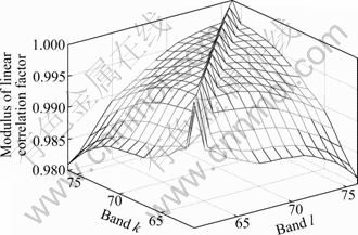
Fig.1 Modulus of linear correlation factor of high frequency curvelet coefficients of AVIRIS data Jasper Ridge

According to Ref.[4], the noise level of each band is determined by the hyperspectral imaging system. The noise variance at a given band varies with the signal level at this band following a predetermined signal-to- noise ratio (SNR) pattern. Some bands are seriously noisy, while some are nearly noise-free. And which band is noisy and which is noise-free is determined by the imaging instrument. Bands at close wavelengths have similar profile structure which can be well captured by curvelet transform. And as mentioned above, the high frequency curvelet coefficients at close wavelengths have strong linear correlation. With this insight, linear interpolation in high frequency coefficients of the noise-free bands can be used to recover the junk bands.

Let f₀, f_L+1 be the noise-free bands, and let the Band f_l, l=1, 2, …, L be the junk bands which need to be recovered. Let λ_l be the wavelength of each band, l=0, 1, …, L+1.

Let W₀, W_L+1 be the sets of high frequency curvelet coefficients in Band f₀ and Band f_L+1, respectively, and let W_l be the set of the linear interpolation of W₀ and W_L+1:

                            (3)

Then, W_l is considered to be a good approximation of high frequency curvelet coefficients in junk bands. The high frequency curvelet transform coefficients in junk bands will be replaced with W_l to recover the profiles of the junk bands.

The junk band recovery algorithm is as follows.

1) Input hyperspectral image data f_l, l=0, 1, …, L+1;

2) Perform curvelet transform on band f_l, l=0, 1, …, L+1;

3) For l=1, 2, …, L, calculate the linear interpolation:

;

4) For l=1, 2, …, L, replace the high frequency coefficients of the junk bands with W_l;

5) For l=1, 2, …, L, inversely transform the curvelet coefficients, and output the recovered image

4 Experimental results

The experimental data are collected by airborne visible/infrared imaging spectrometer (AVIRIS), which is designed by Jet Propulsion Laboratory (JPL), National Aeronautics and Space Administration (NASA). The wavelength of AVIRIS data ranges from 0.4 to 2.45 μm, with a spectral resolution of 10 nm. Each scene has 224 bands. The size of each band is 614 (width)×512 (height). Each pixel occupies 16 bits. Scenes of Jasper Ridge, Lunar Lake and Low Altitude are chosen to test this method. In order to accommodate hyperspectral data cubes in a form that is consistent with the form used in eight-bit images, the test data cubes are rescaled to 8 bits (maximum of 255). The data cubes are extracted from Band 61-76, corresponding to the wavelength of 1.0-1.15 μm, with the size of 256 (width)×256 (height)× 16 (band). Band 61 and Band 76 are taken as noise free bands. Band 62 to Band 75 are taken as junk bands added with Gauss white noise variance of 30. Then, the performance of the algorithm will be estimated objectively and subjectively.

The peak-signal-to-noise ratio (PSNR) is used to estimate the recovering performance objectively. This index reflects the numerical similarity between the recovered image and original image. The PSNR of Band l is defined as

                        (4)

where  denotes the original image pixel at the coordinate (i, j) in Band l.  denotes the recovered image pixel at the coordinate (i, j) in Band l. M and N denote the width and the height of each band, respectively, and L denotes the number of total bands.

The root of mean square error (RMSE) is defined as

                            (5)

The algorithm programs are compiled and run in MATLAB 7.0.1. To show the superiority of this method, the results are compared with a classical image denoising method BayesShrink [8]. This method recovers the junk bands more efficiently than the BayesShrink. Figure 2 shows the PSNR of all recovered bands. Method based on the curvelet achieves higher PSNR. Table 1 lists the comparison of average PSNR and RMSE. To show the advantage of curvelet in this method, wavelet of 8 dB instead of curvelet in the recovery scheme is also taken. The Experimental results in Fig.2 and Table 1 show that this method performs much better than method based on the wavelet. We also compare our method with Curvelet Shrinkage [13]. Our method outperforms well.

A subjective comparison is also given. Taking the band at the wavelength of 1 050 nm for example, Figs.3-5 show the original image, noisy image and recovered image by the BayesShrink, the method based on wavelet, Curvelet shrinkage and this method. Due to the soft thresholding by BayesShrink, the recovered images are blurred at the profiles and edges. The method based on wavelet of 8 dB performs better, but not clear enough at the edges. In this method, the high frequency curvelet coefficients are replaced in the junk bands of the weighted sum of coefficients in the noise-free bands, which recovers the profiles of the junk bands well and keeps the main spectral information unchanged at the same time.

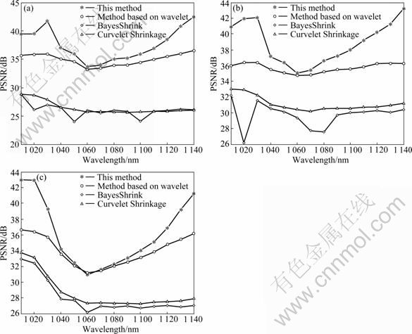
Fig.2 Comparison of recovered band PSNR among this method, method based on wavelet and BayesShrink: (a) Jasper Ridge; (b) Lunar Lake; (c) Low Altitude

Table 1 Average PSNR and RMSE

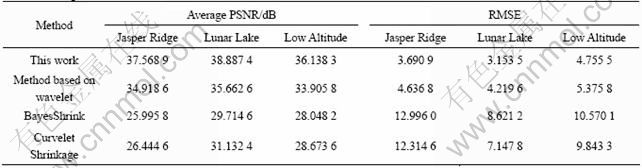
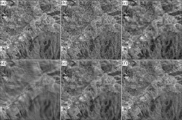
Fig.3 Subjective comparison of recovered band at wavelength of 1 050 nm for Jasper Ridge: (a) Original image; (b) Noisy image;  (c) BayesShrink; (d) Curvelet Shrinkage; (e) Method based on wavelet; (f) This method

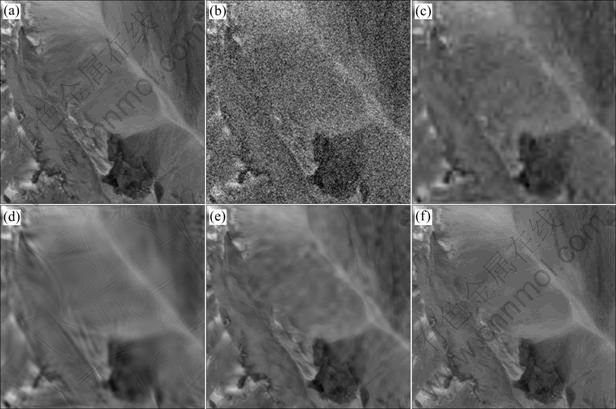
Fig.4 Subjective comparison of recovered band at wavelength of 1 050 nm for Lunar Lake: (a) Original image; (b) Noisy image;   (c) BayesShrink; (d) Curvelet Shrinkage; (e) Method based on wavelet; (f) This method

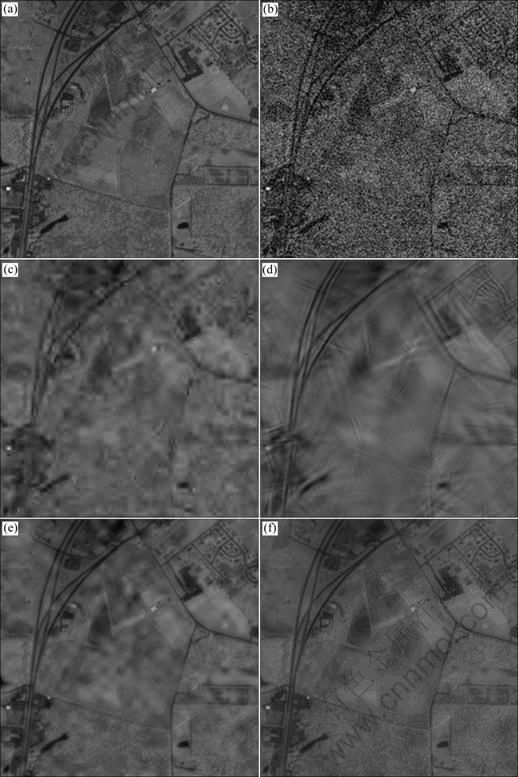
Fig.5 Subjective comparison of recovered band at wavelength of 1 050 nm for Low Altitude: (a) Original image; (b) Noisy image;  (c) BayesShrink; (d) Curvelet Shrinkage; (e) Method based on wavelet; (f) This method

5 Conclusions

1) A hyperspectral image junk band recovery method is proposed based on curvelet transform and the significant spectral correlation.

2) The advantages of this method are as follows. The weighed sum of high frequency coefficient method can avoid distorting the spectral information of the junk bands. It recovers the profiles of the junk bands well.

3) The method is spurious to the classical wavelet threshold method and has wide applications in spectroscopy and spectral analysis.

References

[1] GREEN R O, EASTWOOD M L, SARTURE C M, CHRIEN T G, ARONSSON M, CHIPPENDALE B J, FAUST J A, PAVRI B E, CHOVIT C, SOLIS M, OLAH M R. Imaging spectroscopy and the airborne visible/infrared imaging spectrometer (AVIRIS) [J]. Remote Sensing of Environment, 1998, 65: 227-248.

[2] TONG Qing-xi, ZHANG Bing, ZHENG Lan-fen. Hyperspectral remote sensing-principle: Technology and application [M]. Beijing: Higher Education Press, 2006: 2-6. (in Chinese)

[3] MATES D M, ZWICH H, JOLLY G, SCHULTEN D. System studies of a small satellite hyperspectral mission: Data acceptability [R]. Canada: Can Gov Contract Rep, 2004.

[4] OTHMAN H, QIAN S E. Noise reduction of hyperspectral imagery using hybrid spatial-spectral derivative-domain wavelet shrinkage [J]. IEEE Transactions on Geoscience and Remote Sensing, 2006, 44(2): 397-408.

[5] KAEWPIJIT S, LEMOIGNE J, ELGHAZAWI T. A wavelet-based PCA reduction for hyperspectral Imagery [C]// IEEE International Geoscience and Remote Sensing Symposium. Canada, 2002: 2581- 2583.

[6] SHAH C A, WATANACHATURAPORN P, VARSHNEY P K. Some recent results on hyperspectral image classification [C]// IEEE Workshop on Advance in Technology for Analysis of Remotely Sensed Data. USA, 2003: 346-353.

[7] DONOHO D L. De-noising by soft-thresholding [J]. IEEE Transactions on Information Theory, 1995, 41: 613-627.

[8] CHANG S G, YU B, VETTERLI M. Adaptive wavelet thresholding for image denoising and compression [J]. IEEE Transactions on Image Process, 2000, 9(9): 1532-1546.

[9] PORILLA J, STRELA V, WAINWRIGHT M J, SIMONCELLI E P. Image denoising using scale mixtures of Gaussians in the wavelet domain [J]. IEEE Transactions on Image Processing, 2003, 12(11): 1338-1351.

[10] SHUI P. Image denoising using 2-D separable oversampled DFT modulated filter banks [J]. IET Image processing, 2009, 3(3): 163-173.

[11] ZELINSKI A C, GOYAL V K. Denoising hyperspectral imagery and recovering junk bands using wavelets and sparse approximation [C]// IEEE International Geoscience and Remote Sensing Symposium. USA, 2006: 387-390.

[12] WU Chuan-qing, TONG Qing-xi, ZHENG Lan-fen. De-noise of hyperspectral image based on wavelet transformation [J]. Remote Sensing Information, 2005(4): 10-12. (in Chinese)

[13] CANDES E J, DONOHO D L. Curvelets—A surprisingly effective non-adaptive representation for objects with edges [C]// Proceedings of the in Curve and Surface Fitting. USA, 2000: 105-120.

[14] CANDES E J, DONOHO D L. New tight frames of curvelets and optimal representations of objects with piecewise C² singularities [J]. Comm Pure Appl Math, 2004, 57(2): 219-266.

[15] CANDES E J, DEMANET L, DONOHO D L. Fast discrete curvelet transforms [J]. Multiscale Model Simul, 2006, 5(3): 861-899.

(Edited by YANG Bing)

Foundation item: Project(10871231) supported by the National Natural Science Foundation of China

Received date: 2009-12-04; Accepted date: 2010-07-15

Corresponding author: SUN Lei, PhD; Tel: +86-13548625143; E-mail: bangbangbing1999@163.com