

J. Cent. South Univ. (2019) 26: 1856-1862
DOI: https://doi.org/10.1007/s11771-019-4139-y

A new slope optimization design based on limit curve method
FANG Hong-wei(����ΰ)1,2, CHEN Yohchia(����)3,4, DENG Xiao-wei(����ε)5
1. School of Geomatics and Prospecting Engineering, Jilin Jianzhu University, Changchun 130118, China;
2. School of Civil Engineering and Architecture, Northeast Electric Power University, Jilin 132012, China;
3. School of Civil Engineering, Chongqing University, Chongqing 400045, China;
4. Department of Civil Engineering, The Pennsylvania State University, Middletown PA 17055, USA;
5. Department of Civil Engineering, The University of Hong Kong, Pokfulam, Hong Kong 999077, China
 Central South University Press and Springer-Verlag GmbH Germany, part of Springer Nature 2019
Abstract:
A new method is proposed for slope optimization design based on the limit curve method, where the slope is in the limit equilibrium state when the limit slope curve determined by the slip-line field theory and the slope intersect at the toe of the slope. Compared with the strength reduction (SR) method, finite element limit analysis method, and the SR method based on Davis algorithm, the new method is suitable for determining the slope stability and limit slope angle (LSA). The optimal slope shape is determined based on a series of slope heights and LSA values, which increases the LSA by 2.45��C11.14�� and reduces an invalid overburden amount of rocks by 9.15%, compared with the space mechanics theory. The proposed method gives the objective quantification index of instability criterion, and results in a significant engineering economy.
Key words:
slope optimization design; limit state; limit curve method; limit slope angle��
Cite this article as:
FANG Hong-wei, CHEN Yohchia, DENG Xiao-wei. A new slope optimization design based on limit curve method [J]. Journal of Central South University, 2019, 26(3): 1856-1862.
DOI:https://dx.doi.org/https://doi.org/10.1007/s11771-019-4139-y1 Introduction
Slope optimization design is important for open pits and water dumps, whose main objective is to determine the slope angle under a limit state. This issue has been studied in many countries [1, 2]. Currently, there are three optimization methods available. The first one is the graph theory. KHALOKAKAIE et al [3] developed a computer program for optimal design of open pits based on Lerchs-Grossmann algorithm. RASSAM et al [4] studied three-dimensional (3D) effects on the slope stability of high waste rock dumps and found that the concave surface was stable at an angle at least 2�� steeper than an identical slope following a straight line. The second optimization method is the comprehensive evaluation method. LAI et al [5] adopted a 3D physical model to optimize an open pit excavation by using the acoustic emission sensors with crack optical acquirement and ground penetrating radar and found that the slope angle on the downside was bigger than that on the upside. BYE et al [6] designed an open pit by adopting the mining rock mass rating system (MRMR) and performed numerical simulations using the software FLAC [7] and found that the slope angle deceased with an increasing slope height. SINGH et al [8] assumed a slope angle to perform the limit equilibrium analyses and numerical simulations using (FLAC) to determine the optimal slope angle. CAI et al [9] adopted geographic information system (GIS) based on a 3D limit equilibrium analysis to optimize the slope geometry. MALEKI et al [10] employed an empirical method using the software Phase2D [11] to optimize the slope angle and check the slope stability. LU et al [12] developed a comprehensive method based on the engineering analogy, limit equilibrium, and emulations. The third optimization method is some new techniques as follows. WU et al [13] proposed a new safety cleaning bank mode which reduced an invalid overburden amount of rocks by 3%�C5%. ZHU et al [14, 15] proposed the space mechanics theory (SMT) for slope optimization design, it is shown that the deeper the furrow pit is excavated, the greater the stable slope angle is. Based on the literature survey, the key for the slope optimization design is the determination of the slope under a limit state [16].
The slip-line field theory [17, 18] can determine limit slope load, limit slope height [19] and limit slope curve (LSC) [20]. VO et al [21] developed the stability charts for curvilinear slopes based on the slip-line field theory. FANG et al [22] found a rule based on the relative position between the LSC and the slope, which is a limit curve method (LCM) capable of checking the slope stability. A new method is proposed based on the LCM to calculate the limit slope angle (LSA) and slope optimization design in this work.
2 Description of new method
2.1 Boundary conditions and calculation formula of LSC
This section describes the LSC which is calculated from the slip-line field theory. Only the boundary conditions and calculation formulas pertaining to the LSC are presented in this work as the derivation details have been reported by SOKOLOVSKI [17] and CHEN [18].
According to the slip-line field theory, the slip line can be divided into two families, �� and ��. Their intersection points involve four main parameters, x, y, �� and ��, where x and y are the coordinates, q is the intersection angle between the maximum principal stress (s1) and x axis and s is the characteristic stress. The intersection of slip lines, M (x, y, ��, ��), can be determined by Eqs. (1)�C(4), where M�� (x��, y��, ����, ����) is a point on �� family slip line and M�� (x��, y��, ����, ����) is a point on �� family slip line, m (=��/4�C��/2) is the mean intersection angle between a and b slip lines, and �� is the internal friction angle of soil.
 (1)
(1)
 (2)
(2)

 (3)
(3)
 (
(4)
Note that Eqs. (2) and (4) yield the same result. In determining the LSC, the origin of the Cartesian coordinate system is set at the top of slope with positive x0 axis going rightward and positive y0 axis going downward. While in determining the intersection (i.e., coordinate x1) between the LSC and x axis, the origin of the coordinate system is shifted to the slope toe with positive x axis going rightward and positive y axis going upward, as shown in Figure 1.
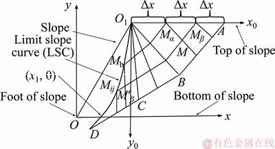
Figure 1 Determination of LSC and x1
The slip-line field theory defines the slope with three zones:
1) Active zone (i.e., O1AB in Figure 1). For the known boundary points on O1A line, Ma and Mb, y=0, and x=��x��i (i=0-N1) with ��x being the calculation step size and N1 being the number of steps. Larger N1 value consumes more computation time. N1=999 is taken in this study based on the computer capability. The intersection angle qI between s1 and x0 axis is ��/2, where  with P as the load at the top of slope.
2) Transition zone (i.e., O1BC in Figure 1). For the known boundary point O1, 
 where
where  with k=0�CN2, ����=��III�C��I, and N2 is the number of transition zone points, qIII is the intersection angle between s1 and x axis in passive zone at point O1.
3) Passive zone (i.e., O1CD in Figure 1). The point on the LSC (i.e., O1D line in Figure 1), Mij(xij, yij, ��ij, ��ij), can be determined by Eqs. (5)�C(8), where M����(x����, y����, �ȡ���, �ҡ���) is the known point on b slip line and Mb(xb, yb, ��b, ��b) is the known point on the LSC. The first Mb point is the origin at the top of slope (i.e., point O1), which has xb=0, yb=0, 
 and ��b=��III=
  with c=cohesion.
 (5)
(5)
 (6)
(6)


 (7)
(7)
 (8)
(8)
Note that Eq. (6) yields the same result. To satisfy  the minimum load at the top of slope
  When there is no external load on the slope, the minimum load is imposed at the top of slope to advance the calculation. As such, the value of N2 has no effect on the calculation results and it is hence set equal to zero in this study.
2.2 Proposed method based on LCM
The new method based on LCM [22] is defined as: stable condition when x1>0 (x1 being the abscissa of the intersection between the LSC and the bottom of slope); limit state condition when x1=0; unstable condition when x1<0 (Figure 2). A computer program utilizing MATLAB [23] was developed by the authors to facilitate the computations using Eqs. (1)�C(4) and (5)�C(8).
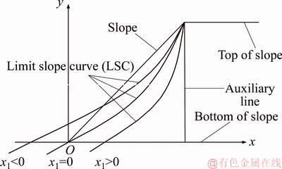
Figure 2 New method based on LCM
2.3 Proof of new method
The new method is combined with the SRM [24] to determine the factor of safety (FOS) against the slope stability. The flowchart of the proposed computation method is shown in Figure 3.
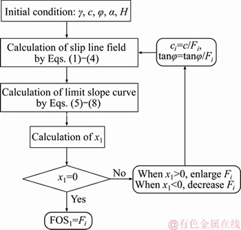
Figure 3 Flowchart for calculation of safety factor by proposed method
Material set 2 of the case described by TSCHUCHNIGG et al [25] was adopted in this study to calculate the safety factors (SFs) along with unit weight ��=19 kN/m3, cohesion c=20 kPa, friction angel ��=25��, slope height H=10 m, and slope angle ��=15��C60��.
The computed SFs by TSCHUCHNIGG et al [25] and the proposed method are listed in Table 1. In the table, SRFEA1 and FELA1 are respectively the strength reduction (SR) method and finite element (FE) limit analysis method under the ��associated flow rule��, SRFEA2 and FELA2 are respectively the SR method and FE limit analysis method under the ��non-associated flow rule��, and SRFEA (Davis) represents the SR method based on Davis algorithm [25]. It shows that the SFs by all methods decrease with increasing �� value. Relative errors (E) for the SFs and Pmin values are summarized in Table 2, which are calculated by
 (9)
(9)
Table 1 Comparison of SFs
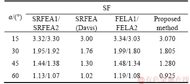
The proposed method yields 5.99%�C18.14% lower SFs than the SR method and �C1.32%�C 22.27% lower SFs than the FE limit analysis method (Table 2). The computed SFs between the proposed method and the SRFEA (Davis) method are similar. Note that higher Pmin value implies lower slope stability and smaller slope safety factor. Relative errors increase with increasing Pmin values. The main advantages of the proposed method are that there is no need to assume or search for a critical slip surface to determine if the slope is in a limit state, and it gives the objective quantification index of instability criterion.
Table 2 Relative errors of SFs and Pmin

3 Slope optimization design
3.1 Calculation of limit slope angle (LSA)
The following new method is proposed to calculate the limit slope angle (LSA, Acs): Increasing the slope angle a with constant c and j values, when the limit slope curve (LSC) and the slope intersect at the toe of the slope (i.e., x1 = 0), the corresponding a is the LSA, as shown Figure 4. The computational flowchart for the LSAs is shown in Figure 5.

Figure 4 Calculation of LSAs (a1<>2<>3):
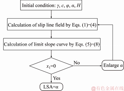
Figure 5 Flowchart for calculation of LSAs by proposed method
The case of TSCHUCHNIGG et al [25] described in Section 2.3 was used. The analysis results show that with an increasing ��, the relative position relation between the LSC and the slope line changes from separation to intersection, as shown in Figure 6. At x1=0, the calculated LSA value by the proposed method is 56.7�� versus the approximate 60�� by the SRFEA(Davis) method, as shown in Table 1, with an error of 5.5%.
3.2 Comparison with space mechanics theory
The slope optimization can be achieved through the determination of LSA as: for a specific H value, increase a to the LSA until x1=0 (i.e., a slope limit state) is reached; based on the series of H and LSA values, determine the optimal slope shape using the MATLAB function ��plot��. ZHU et al [14, 15] proposed the space mechanics theory (SMT) for slope optimization design according to the limit equilibrium principle, in which the relation between H and r (the set horizontal distance for the SMT) is shown in Eq. (4). The LSA is then calculated by Eq. (5), where r0 is set at 100 m.

 (9)
(9)
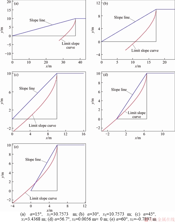
Figure 6 Calculated LSAs by proposed method:
 (10)
(10)
where r1 is the horizontal distance for the proposed method determined by Eq. (6) in which ALS1 is the limit slope angle calculated by the proposed method.
 (11)
(11)
The comparison of LSA values between the SMT and the proposed method is shown in Table 3, in which ��=27 kN/m3, c=200 kPa and ��=45�� are assumed [15]. It shows that the proposed method increases LSA values by 2.45��C11.14��. The comparison of slope optimization designs is shown in Figure 7 with the first coordinates of r0=100 m and H=0 m at the foot of slope, point A is the foot of slope, points B and C are the top of slope determined respectively by the proposed method and the SMT, and points E and D are the bottom of slope determined respectively by the proposed method and the SMT. The results show that the optimal slope determined by the proposed method is a convex curve that is relatively flat in the upper portion and rather steep in the lower portion (i.e., an up flat-down steep curve). The reduced invalid overburden amount of rocks is 9.15%=SABC/SACD= (SABE+SBCDE�CSACD)/SACD, where SABE+SBCDE is the amount of rocks calculated by the proposed method and SACD is the amount of rocks calculated by the SMT.
Table 3 Comparison of LSAs

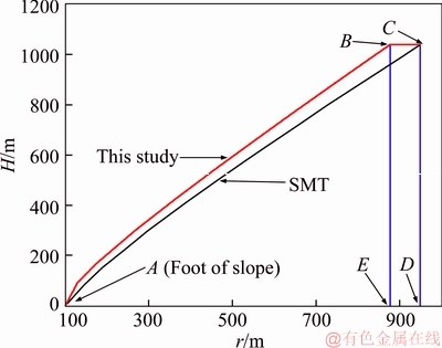
Figure 7 Comparison of slope optimization design
4 Conclusions
A new method for slope optimization designs is proposed, which is based on the limit curve method. The slope is in the limit equilibrium state when the limit slope curve calculated from the slip-line field theory and the slope intersects at the toe of the slope. The safety factors for stability computed by the proposed method are found to generally match with those calculated by the SRFEA method. The analysis results show that the relative position relation between the LSC and the slope line changes from separation to intersection with an increasing slope angle. The relative error between the calculated LSA value by the proposed method and that of the SRFEA (Davis) method is merely 5.5%. The proposed method need not require knowing a critical slip surface in advance when determining if the slope is in a limit state and gives the objective quantification index of instability criterion.
The calculated limit slope angles (LSAs) by the proposed method is 56.7�� which is close to 60�� computed by the SRFEA (Davis) method. Based on the computed various slope heights H and LSA values, an optimal slope shape can then be determined through the use of MATLAB function ��plot��. The optimal slope shape by the proposed method is convex, indicating that the computed LSA values increase with decreasing H values. Compared with the space mechanics theory, the proposed method increases the LSA by 2.45��C11.14��, resulting in 9.15% reduction of invalid overburden rocks, which is economically beneficial.
References
[1] MELNIKOV N N,KOZYREV A A, RESHETNYAK S P,KASPARIAN E V, RYBIN V V. Geomechanical and technical substantiation of an optimal slope angle in the kovdor open pit [R]. International Symposium on Mining in the Arctic.2003: 321�C326.
[2] LI Y, YANG S, ZHONG F S. Rock slope angle optimization based on finite element method and limit equilibrium theory [J]. China Safety Science Journal, 2012, 22(2): 145�C150. (in Chinese)
[3] KHALOKAKAIE R, DOWD P A, FOWELL R J. A Windows program for optimal open pit design with variable slope angles [J]. International Journal of Surface Mining, Reclamation and Environment, 2000, 14(4): 261�C275.
[4] RASSAM D W, WILLIAMS D J. 3-Dimensional effects on slope stability of high waste rock dumps [J]. International Journal of Surface Mining, Reclamation and Environment, 1999, 13(1): 19�C24.
[5] LAI X P, SHAN P F, CAI M F, REN F H, TAN W H. Comprehensive evaluation of high-steep slope stability and optimal high-steep slope design by 3D physical modeling [J]. International Journal of Minerals, Metallurgy and Materials, 2015, 22(1): 1�C11.
[6] BYE A R, BELL F G. Stability assessment and slope design at Sandsloot open pit, South Africa [J]. International Journal of Rock Mechanics & Mining Sciences, 2001, 38: 449�C466.
[7] Itasca Consulting Group, INC. User��s manual for FLAC3D (Fast Lagrangian Analysis of Continua in 3 Dimensions), Version 3.0 [M]. Twin Cities, USA: The Itasca Consulting Group, Inc., University of Minnesota, 2003.
[8] SINGH V K, SINGH J K, KUMAR A. Geotechnical study for optimizing the slope design of a deep open-pit mine, India [J]. Bull Eng Geol Environ, 2005, 64(3): 303�C309.
[9] CAI M F, XIE M W, LI C L. GIS-based 3D limit equilibrium analysis for design optimization of a 600 m high slope in an open pit mine [J]. Journal of University of Science and Technology Beijing, 2007, 14(1): 1�C5.
[10] MALEKI M R, MAHYAR M, MESHKABADI K. Design of overall slope angle and analysis of rock slope stability of Chadormalu Mine using empirical and numerical methods [J]. Engineering, 2011, 3(9): 965�C971.
[11] ROCSCIENCE INC. User��s manual for Phase2D (a 2D finite element program for stress analysis and support design around excavations in soil and rock) [M]. Toronto, Canada: The Rocscience Inc., 2014.
[12] LU Z L, WU L, YUAN Q, LI B. Open-pit slope optimal angle of bong peak mining based on EALEE comprehension method [J]. Electronic Journal of Geotechnical Engineering, 2013,18: 4263�C4280.
[13] WU A X, JIANG L C, BAO Y F, LI J F. Stability analysis of new safety cleaning bank in steep slope mining [J]. Journal of Central South University, 2004, 11(4): 423-428.
[14] ZHU N L, ZHANG S X. Determination of the stable slope configuration of oval-shaped furrow pits [J]. Journal of Wuhan University of Technology-Mater Sci Ed, 2004, 19(1): 86�C88.
[15] ZHU N L, ZHANG S X. A basic way to determine the stable slope angle for furrow pits [J]. Engineering Mechanics, 2003, 20(5): 130�C133. (in Chinese)
[16] CARL T, INTRIERI E, FARINA P, CASAGLI N. A new method to identify impending failure in rock slopes [J]. International Journal of Mechanics & Mining Sciences, 2017, 93: 76�C81.
[17] SOKOLOVSKI V V. Statics of granular media [M]. Oxford, UK: Pergamon Press, 1965.
[18] CHEN Z. Granular materials limit equilibrium theory foundation [M]. Beijing: Hydraulic Publisher, 1987. (in Chinese)
[19] FREDLUND D G. State-of-the-Art: Analytical methods for slope stability analysis [C]// Proceedings of the Fourth International Symposium on Landslides. Toronto, Canada, 1984: 229�C250.
[20] JELDES I A, VENCE N E, DRUMM E C. Approximate solution to the Sokolovski concave slope at limiting equilibrium [J]. Int J Geomech, 2013, 15(2): 1�C8.
[21] THANH V, RUSSELL A R. Stability charts for curvilinear slopes in unsaturated soils [J]. Soils Found, 2017, 57(4): 543�C556.
[22] FANG H W, LI C H, LI B. Limit curve method of homogeneous slope stability [J]. Rock and Soil Mechanics, 2014, 35(S1): 156�C164. (in Chinese)
[23] MATHWORKS INC. User��s manual for MATLAB (programming fundamentals) [M]. Natick, Massachusetts, USA: The Mathworks Inc., 2009.
[24] GRIFFITHS D V, LANE P A. Slope stability analysis by finite elements [J]. Geotechnique, 1999, 49(3): 387�C403.
[25] TSCHUCHNIGG F, SCHWEIGER H F, SLOAN S W, LYAMIN A V, RAISSAKIS I. Comparison of finite-element limit analysis and strength reduction techniques [J]. Geotechnique, 2015, 65(4): 249�C257.
(Edited by FANG Jing-hua)
���ĵ���
һ���µĻ��ڼ������߷��ı����Ż���Ʒ���
ժҪ�����ڼ������߷������һ���µı����Ż���Ʒ��������ɻ����߳����ۼ���ļ���״̬�µı���������������������ཻ���½�ʱ���жϱ��´��ڼ���״̬���봫ͳ��ǿ���ۼ���������Ԫ��������������Davis�㷨��ǿ���ۼ�����Աȣ�����ķ��������ڼ��㼫���½ǡ������������������¸ߺ��½ǵõ��ı����Ż����棬��ռ�������Աȣ��½������2.45��~11.14�㣬��ʡ����Ͽ����������9.15%������ķ��������˱���ʧ�ȵĿ�����ָ�꣬�ܹ�����������ľ���Ч�档
�ؼ��ʣ������Ż���ƣ�����״̬���������߷��������½�
Foundation item: Project(JJKH20180450KJ) supported by Education Department of Jilin Province, China; Project(20166008) supported by the Science and Technology Bureau of Jilin Province, China
Received date: 2018-01-10; Accepted date: 2018-10-15
Corresponding author: CHEN Yohchia, PhD, Professor; Tel: +86-17179486146; E-mail: yxc2@psu.edu
Abstract: A new method is proposed for slope optimization design based on the limit curve method, where the slope is in the limit equilibrium state when the limit slope curve determined by the slip-line field theory and the slope intersect at the toe of the slope. Compared with the strength reduction (SR) method, finite element limit analysis method, and the SR method based on Davis algorithm, the new method is suitable for determining the slope stability and limit slope angle (LSA). The optimal slope shape is determined based on a series of slope heights and LSA values, which increases the LSA by 2.45��C11.14�� and reduces an invalid overburden amount of rocks by 9.15%, compared with the space mechanics theory. The proposed method gives the objective quantification index of instability criterion, and results in a significant engineering economy.
