
J. Cent. South Univ. (2012) 19: 1240-1248
DOI: 10.1007/s11771-012-1135-x![]()
A nonlinear bottom-following controller for underactuated autonomous underwater vehicles
JIA He-ming(�ֺ���)1,2, ZHANG Li-jun(������)3, BIAN Xin-qian(����ǭ)2, YAN Zhe-ping(����ƽ)2,
CHENG Xiang-qin(������)2, ZHOU Jia-jia(�ܼѼ�)2
1. College of Mechanical and Electrical Engineering, Northeast Forestry University, Harbin 150040, China;
2. College of Automation, Harbin Engineering University, Harbin 150001, China;
3. School of Marine Engineering, Northwestern Polytechnical University, Xi��an 710072, China
? Central South University Press and Springer-Verlag Berlin Heidelberg 2012
Abstract:
The bottom-following problem for underactuated autonomous underwater vehicles (AUV) was addressed by a new type of nonlinear decoupling control law. The vertical bottom-following error and pitch angle error are stabilized by means of the stern plane, and the thruster is left to stabilize the longitudinal bottom-following error and forward speed. In order to better meet the need of engineering applications, working characteristics of the actuators were sufficiently considered to design the proposed controller. Different from the traditional method, the methodology used to solve the problem is generated by AUV model without a reference orientation, and it deals explicitly with vehicle dynamics and the geometric characteristics of the desired tracking bottom curve. The estimation of systemic uncertainties and disturbances and the pitch velocity PE (persistent excitation) conditions are not required. The stability analysis is given by Lyapunov theorem. Simulation results of a full nonlinear hydrodynamic AUV model are provided to validate the effectiveness and robustness of the proposed controller.
Key words:
underactuated autonomous underwater vehicle; bottom-following; nonlinear iterative sliding mode��
1 Introduction
With the fast progresses of the marine robotics, the autonomous underwater vehicles (AUVs) need a bottom navigation ability to follow the bottom profile at a constant altitude as a basic feature for successful undersea search and survey, maritime reconnaissance, communication/navigation aids, and tracking and trailing in uncharted shallow water [1]. In recent years, voluminous literatures have been presented on the subject of designing bottom-following controllers for AUVs [2-10]. The underlying difficulties for bottom- following problem are that some AUVs have fewer actuators than degrees of freedom to be controlled, and the nonholonomic systems cannot track arbitrary trajectories. The uncertain dynamics and drift caused by unknown ocean currents make this problem even intractable.
The type of AUV considered in this work is equipped with two identical back thrusters mounted symmetrically with respect to its longitudinal axis. Especially, the vehicle is underactuated since it lacks any vertical thruster. The common and differential modes of the thrusters generate a force along the longitudinal axis of the vehicle and the pitch rudder produces a torque about its vertical axis. In this work, a full dynamic model of an AUV operated by the Best Sea Assembly Institute of Harbin Engineering University, China, will be used.
In order to deal with the problem that the arbitrary trajectories tracking control of underactuated AUVs is influenced by the nonholonomic constraint on accelerations, some researchers concentrate their interests on the applications of reference model method to this control problem [11-13]. To design the bottom-following controller using this method, the desired reference orientation (pitching angle) must be computed and higher order derivatives need to be generated by a reference model. However, in practice, motions of AUV are very complicated, and environmental disturbance such as shallow water and currents may have very strong effects on the maneuverability. So, the hydrodynamic model of a AUV is highly nonlinear, complex and uncertain, and it is infeasible to generate a desired reference trajectory by an accurate model. This work is without a reference orientation generated by a AUV model, and it has more advantages than the traditional reference model method, because it deals explicitly with vehicle dynamics and the geometric characteristics of the desired tracking bottom curve. In Ref. [11], a similar technique was firstly proposed for path-following problem of an underactuated AUV. This design procedure effectively creates an extra degree of freedom that can then be explored to avoid the singularities that occur when the distance to path is not well defined (this occurs for example when the vehicle is located exactly at the center of curvature of a circular path).
In the previous study [12], an iterative nonlinear sliding mode (INSM) geometrical path following controller was proposed with the control input of rudder deflection alone for an underactuated surface ship under uncertain perturbation of the disturbances, and the main thruster was left free. Compared with traditional high-order sliding mode control (SMC) strategy, iterative nonlinear sliding mode control (INSMC) has great advantages. The proposed control algorithm is easy to be implemented based on engineering design problem, so the control law can be realized easily for real application.
In the present work, the INSM integrated with simple increment feedback control method is extended to bottom-following and speed adjusting using decoupling control method for an underactuated AUV. The estimation of systematic uncertainties and environmental disturbances and the pitch velocity persistent excitation (PE) conditions are not required. Furthermore, in order to better meet the need of engineering applications, the working characteristics of actuators are explicitly involved in the design of controller.
2 Problem formulation
2.1 Vehicle modeling: Kinematics and dynamics
The kinematic equations of the AUV can be written as [13]
 (1)
(1)
Assuming that u is never equal to zero, the reference frame W that is obtained from B by rotating it around the yB axis through angle �� in the positive direction is considered. The above equation can then be rewritten to yield
 (2)
(2)
where ��W=��B+��. Clearly, ![]() . Neglecting the equations in sway, roll and yaw, the simplified equations for surge, heave and pitch can be written as [14-15]
. Neglecting the equations in sway, roll and yaw, the simplified equations for surge, heave and pitch can be written as [14-15]
 (3)
(3)
where

2.2 Bottom following: Error coordinates
The solution to the problem of bottom following proposed here is built on the following intuitive explanation [16-17] (see Fig. 1): A simple bottom- following controller should compute: 1) the distance between the vehicle��s center of mass Q and the closest point P on the Path 1, and 2) the angle between the vehicle��s total velocity vector ��t and the tangent to the Path 1 at P, and both reduce to zero. This motivates the development of the ��kinematic�� model of the vehicle in terms of a Serret-Frenet frame F that moves along the path; F plays the role of the body axis of a ��virtual target vehicle�� that should be tracked by the ��real vehicle��. Using this set-up, the above mentioned distance and angle become the coordinates of the error space where the control problem is formulated and solved. In this work, however, a Frenet frame F that moves along the bottom path to be followed is used with a significant difference: the Frenet frame is not attached to the point on the path that is closest to the vehicle. Instead, the origin OF=P of F along the path is made to evolve according to a conveniently defined control law, effectively yielding an extra controller design parameter. As will be seen, this seemingly simple procedure is instrumental in lifting the stringent initial condition constraints that are presented in Ref. [18] for path following of marine vehicles.
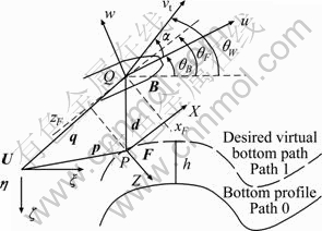
Fig. 1 Schematic diagram of bottom following: Reference frames
Consider Fig. 1, where P is an arbitrary point on the Path 1 to be followed. Associated with P, consider the corresponding Serret-Frenet frame F. The signed curvilinear abscissa of P along the path is denoted as ��. Clearly, Q can either be expressed as q=[x, 0, z]T in U or as [xF, 0, zF]T in F. Stated equivalently, Q can be given in (x, z) or (xF, zF) coordinates. Let

be the rotation matrix from U to F, parameterized locally by the angle ��F. Define ![]() , then
, then
![]() (4)
(4)
where cc(��) and gc(��) denote the path curvature and its derivative, respectively. The velocity of P in U can he expressed in F to yield
![]()
The velocity of Q in U can be expressed in F as
![]() (5)
(5)
where d is the vector from P to Q.
Using the relations

Eq. (5) can be rewritten as
![]() (6)
(6)
Finally, replacing the top two equations of Eq. (2) in Eq. (6) and introducing the variable ��=��W-��F and ![]() give the ��kinematic�� model of the AUV in (xF, zF) coordinates as
give the ��kinematic�� model of the AUV in (xF, zF) coordinates as
 (7)
(7)
2.3 Model of actuators
The forward speed of the underactuated AUV is controlled by two identical back propeller thrusters. The related rotating speed equation is[20]
![]() (8)
(8)
where KM is the control gain of the thruster, N is the rotating speed of the thruster, Nr is the rotating speed command, and TM is the time constant of the thruster.
The rudder actuator model is [20]
![]() (9)
(9)
where KE is the control gain of the rudder, �� is the rudder angle, ��r is the rudder angle command, and TM is the time constant of the rudder.
2.4 Problem formulation
With the above notations, the problem under study can be formulated as follows.
Consider the AUV model with kinematic and dynamic equations given by Eqs. (1) and (3). Given a desired bottom path to be followed and a desired profile ud(t)>umin>0 for the surge speed u, derive nonlinear feedback control laws for the force Xprop and torque Mprop, and rate of evolution ![]() of the curvilinear abscissa �� of the ��virtual target�� point P along the path so that xF, zF, �� and u-ud tend to be zero asymptotically.
of the curvilinear abscissa �� of the ��virtual target�� point P along the path so that xF, zF, �� and u-ud tend to be zero asymptotically.
3 Nonlinear bottom-following controller design
An iterative nonlinear sliding mode (INSM) control law is introduced to steer the dynamic model of an underactuated AUV described by Eqs. (1)-(3) along a desired bottom path. The merits of application of INSM are to guarantee the robustness of the controller and to avoid uncertainties estimation [19].
3.1 Preliminaries
1) Iterative nonlinear sliding mode (INSM)
For a single input-single output (SISO) system or a decoupled subsystem with a kind of lower triangular form, if the dynamics is continuously differentiable, the iteratively nonlinear sliding mode designing procedure can be described as

where e denotes the output tracking error of the system, n is the order of the system, and k2i-1, k2i��R+(i=1, 2, ��, n). From the definition of ��i, it can be concluded that
if ��n(��n-1)��0,
then
![]() (11)
(11)
Similarly, it can iteratively be deduced that
If ��1(e)��0,
then
![]() (12)
(12)
Thus, the control objective of tracking error e is transformed iteratively into stabilization of ��n, which is defined in the augmented state space. The overall sliding mode system consists of n nested sliding mode controllers that progressively stabilize each outer subsystem. The advantage of recursive and decentralized designing lies in the capability of dealing with uncertainties. And a distinguishing quality may be available since free phase plane trajectories can be designed. For more detailed designing, especially for nonholonomic control systems, one can refer to Ref. [20]. Undoubtedly, there are other switching functions and their associated sliding modes described by differential equations. Notice that the hyperbolic tangent function is strictly bounded and the parameters k2i-1 have clear functional meaning of the upper bound of converging rate of ��i-1, which may be convenient for controller designing and parameters tuning. The performance of the controller can be adjusted by parameter tuning according to prevailing conditions, systematic constraints or even subjectiveness. The parameters k2i serve as coordinate compressors which determine together with k2i-1 the upper bound of the slop of sliding modes ��i-1.
2) Increment feedback
Consider the scalar function ��n defined in Eq. (10). It can be rewritten in the form as
![]() (13)
(13)
where f is defined in x��Rn+1, u��R and t��R+. If ![]() ,
,![]() such that
such that ![]() , where f is an explicitly reversible function, and all independent variables are measurable, then a control law may be explicitly derived. In such a case, designing a control law is just a problem of solving an equation. Unfortunately, this is not true in general. However, under certain conditions, it is possible to design some simple control laws and asymptotical stability or practical stability of the close-loop system can be rendered.
, where f is an explicitly reversible function, and all independent variables are measurable, then a control law may be explicitly derived. In such a case, designing a control law is just a problem of solving an equation. Unfortunately, this is not true in general. However, under certain conditions, it is possible to design some simple control laws and asymptotical stability or practical stability of the close-loop system can be rendered.
Theorem 1: Considering a SISO system with sliding schemes described by Eqs. (10) and (13), there exists a constant scalar kp1>0, such that the increment feedback controller![]() can asymptotically stabilize the close-loop system, if the following conditions hold:
can asymptotically stabilize the close-loop system, if the following conditions hold:
(1) f is Lipschitz in (x, u) and all states and independent variables are bounded;
(2)![]() ,
, ![]() such that f(x(t), u*(t), t)=0;
such that f(x(t), u*(t), t)=0;
(3) ![]() .
.
Proof: Supposing at t=t1, ��n>0, because of condition (3) we can draw a conclusion that u*(t1)![]() When
When ![]() we can conclude that
we can conclude that ![]() and f��0, so the close-loop system is asymptotically stable.
and f��0, so the close-loop system is asymptotically stable.
Theorem 2: Considering a SISO system with sliding schemes described by Eqs. (10) and (13), there exist a constant scalar kp2>0, and an increment feedback controller ![]() such that the close-loop system can be rendered practically stable, if the following conditions hold:
such that the close-loop system can be rendered practically stable, if the following conditions hold:
(1) f is Lipschitz in (x, u) and all states and independent variables are bounded;
(2) ![]() ,
, ![]() such that f(x(t), u*(t), t)=0;
such that f(x(t), u*(t), t)=0;
(3) ![]()
Proof: Supposing at t=t1, ��n>0, because of condition (3) we can draw a conclusion that u*(t1)
Remark 1: Theoretically speaking, the larger the increment feedback gains kp1 and kp2 are valued, the better the controllers perform. However, due to the time lags during the transmission of measurement and control signals, an excess of feedback gain may cause over-sensitiveness and oscillating of the actuators.
3.2 Nonlinear sliding mode schemes
For bottom-following error coordinate system Eq. (7), propeller model Eq. (8) and rudder actuator model Eq. (9) with modeling uncertainties and current disturbances, our dynamic nonlinear sliding mode controller is designed using decoupling control method. The vertical bottom-following error zF and pitch angle error �� can be stabilized by means of the rudder alone, and the thruster is left to adjust the speed and fulfill the control objective of stabilization of the longitudinal bottom-following error xF and the surge speed u.
1) Vertical bottom-following error control
In order to stabilize zF and ��, nonlinear sliding surfaces are designed as
 (14)
(14)
where ![]() ,
, ![]() ,
, ![]() ,
, ![]() ,
, ![]() ��R+. Thus, the control objective of zF and �� is iteratively transformed into stabilization of
��R+. Thus, the control objective of zF and �� is iteratively transformed into stabilization of ![]() .
.
From definition of ![]() ,
, ![]() and
and ![]() , it can be easily concluded that:
, it can be easily concluded that:
If ![]()
then
![]() (15)
(15)
Similarly,
![]() (16)
(16)
and
![]() (17)
(17)
Considering Eqs. (1), (2) ,(3) and (14), we can get
![]() (18)
(18)
In the bottom-following operational condition, if the AUV is proceeded forward(|��|<<��/2 and u>>w), we know that there exists a ��*(t)��(-��/2, ��/2) which satisfies ![]() and
and ![]() .
.
From Eq. (17), we can get
![]() (19)
(19)
Supposing at t=t1,![]() because of
because of ![]() , we can draw a conclusion that ��*(t1)<��(t1). From Eq. (19), we know that �� is continuously decreased owing to the monotony of hyperbolic tangent function. Since the kinematics is smooth and ��*(t) is bounded, if ��*(t) is periodical, there must exist t=t2, t=t3, ��, at which ��=��*, and
, we can draw a conclusion that ��*(t1)<��(t1). From Eq. (19), we know that �� is continuously decreased owing to the monotony of hyperbolic tangent function. Since the kinematics is smooth and ��*(t) is bounded, if ��*(t) is periodical, there must exist t=t2, t=t3, ��, at which ��=��*, and ![]() . So, a practical stability can be achieved. Particularly, if ��*(t)���� as t����, where �� is a constant bottom-following loxodrome, we can conclude that ��(t)����, then
. So, a practical stability can be achieved. Particularly, if ��*(t)���� as t����, where �� is a constant bottom-following loxodrome, we can conclude that ��(t)����, then
![]() (20)
(20)
which means zF exponentially converges to zero with an maximum converging rate determined by ![]() .
.
Remark 2: From the recursive designing procedure including coordinate transformation, it can be seen that it is favorable to select parameters satisfying following inequalities:
![]() (21)
(21)
These parameters can be easily valued according to the maneuverability of AUV because of their clear functional meanings. For example, ![]() denotes the upper bound of pitching rate that the AUV is forced to follow.
denotes the upper bound of pitching rate that the AUV is forced to follow.
Remark 3: To prevent AUV from steering a wrong (backward) way in the bottom-following operational condition, the integration in Eq. (14) can be saturated with ��max (the maximum of pitch leeway or incidence angle) evaluated according to AUV navigational and hydrometeorological conditions of AUV.
2) Longitudinal bottom-following error control
In order to stabilize the longitudinal bottom- following error xF and the surge speed u using thruster, nonlinear sliding surfaces are decentralized and designed in a similar procedure as
 (22)
(22)
where ![]() ,
, ![]() ,
, ![]() ,
, ![]() ��R+. Thus, the control objective of xF and u is iteratively transformed into stabilization of
��R+. Thus, the control objective of xF and u is iteratively transformed into stabilization of![]() .
.
3.3 Feed back control laws
To stabilize ![]() and
and ![]() , robust control laws are needed because of the complicated and uncertain dynamics of AUV and exogenous disturbances. We employ simple increment feedback control laws:
, robust control laws are needed because of the complicated and uncertain dynamics of AUV and exogenous disturbances. We employ simple increment feedback control laws:
 (23)
(23)
According to Eq. (19), the input command of rudder angle and rotating speed can be obtained from the working characteristics of rudder actuator and propeller:
 (24)
(24)
where ![]() ,
, ![]() ,
, ![]() ,
, ![]() ��R+. Without uncertainties estimation, the control laws in Eq. (23) can asympototically stabilize
��R+. Without uncertainties estimation, the control laws in Eq. (23) can asympototically stabilize ![]() and
and ![]() .
.
4 Stability analysis
Theorem 3: According to AUV system Eqs. (1), (2) and (3), with the actuators model Eqs. (8) and (9), according to the AUV bottom-following error Eq. (7), under the designed nonlinear controller Eqs. (14), (22) and (23), all the error states and signals in the bottom-following control system are asymptotically stable.
Proof:
1) Vertical bottom-following error system
Considering the following Lyapunov function: ![]() , the derivative of V1 along Eq. (23) will be
, the derivative of V1 along Eq. (23) will be
![]() (25)
(25)
Expanding ![]() yields
yields
![]()
![]() (26)
(26)
Considering Eqs. (1), (2) ,(3) and (26), we can get
![]() (27)
(27)
Assuming that Mprop is a monotomic function of ��, when the parameter ![]() is properly selected, it can be concluded that
is properly selected, it can be concluded that ![]() .
.
From Eqs. (14), (23) and (25), it follows
![]() (28)
(28)
then ![]() .
.
Based on rudder actuator model Eq. (9), due to the boundedness of hypobolic tangent function, there must exist the appropriate parameters ![]() (i=1, 2, ��, 7) ��R+ and the proper rudder angle command which satisfies
(i=1, 2, ��, 7) ��R+ and the proper rudder angle command which satisfies ![]() On the basis of increment feedback theorem (details of the proof procedure are given in Ref. [16]), assuming that the environmental disturbances are sufficiently smooth, control law Eq. (23) can make
On the basis of increment feedback theorem (details of the proof procedure are given in Ref. [16]), assuming that the environmental disturbances are sufficiently smooth, control law Eq. (23) can make ![]() stable. With the definition of
stable. With the definition of ![]() and
and ![]() , since
, since ![]() ,
, ![]() is negative semi-definition when
is negative semi-definition when ![]() according to the Barbalat lemma [21-22]:
according to the Barbalat lemma [21-22]:![]() as
as ![]() Furthermore, zF and �� will converge to zero according to
Furthermore, zF and �� will converge to zero according to ![]() . As a result, the vertical bottom-following error control system is asymptotically stable.
. As a result, the vertical bottom-following error control system is asymptotically stable.
2) Longitudinal bottom-following error system
Consider the following Lyapunov function ![]() , the derivative of V2 along Eq. (23) will be
, the derivative of V2 along Eq. (23) will be
![]() (29)
(29)
Expanding ![]() yields
yields
![]() (30)
(30)
Neglecting the variables which are unrelated to the rotating speed, the derivative of ![]() along N will be
along N will be
![]() (31)
(31)
Assuming that Xprop is a monotomic function of N, since the AUV cannot track the bottom of seabed in the backward (wrong) way, ensuring ![]() even
even ![]() , then
, then ![]() .
.
From Eqs. (22), (23) and (29), it follows
![]() (32)
(32)
then ![]() .
.
Based on the propeller thruster model Eq. (8), due to the boundedness of hypobolic tangent function, there must exist the suitable parameters ![]() (j=1, 2, ��, 6) ��R+ and the proper thruster rotating speed command which satisfies
(j=1, 2, ��, 6) ��R+ and the proper thruster rotating speed command which satisfies ![]() According to increment feedback theorem [16], assuming that the environmental disturbances are also sufficiently smooth��control law Eq. (23) can make
According to increment feedback theorem [16], assuming that the environmental disturbances are also sufficiently smooth��control law Eq. (23) can make ![]() stable. With the definition of
stable. With the definition of ![]() and
and ![]() , since
, since ![]() ,
, ![]() is negative semi-definition when
is negative semi-definition when ![]() according to the Barbalat lemma [21-22]:
according to the Barbalat lemma [21-22]: ![]() as
as ![]() Furthermore, xF will converge to zero according to
Furthermore, xF will converge to zero according to ![]() As a result, the longitudinal bottom-following error control system is asymptotically stable.
As a result, the longitudinal bottom-following error control system is asymptotically stable.
Remark 4: High frequency (HF) components of disturbances can cause unnecessary wear and tear of the actuators and must be removed by low-pass filter from the vehicle measurements before they enter the control loop [19]. In the present work, the necessary filtering of HF is assumed to have been taken care of in the output measurements.
5 Simulation analyses
The INSM tracking controller presented in the previous sections can be applied to bottom-following for AUVs. In this work, a setup is considered where two narrow beam echo sounders, mounted underneath the AUV, scan the seabed along the vehicle��s direction of forward motion, as shown in Fig. 2. As a result of this setup, a preview-based method can be adopted to build the desired virtual bottom path from measurement data of echo sounders [10].

Fig. 2 Sensor readings to obtain desired virtual bottom path
Table 1 summarizes the key parameters of the AUV model used and the actuators parameters are clearly given in Table 2. The desired virtual bottom path and actual vehicle trajectories with INSM and PID controller are shown in Fig. 3. The PID controller is chosen as
![]()
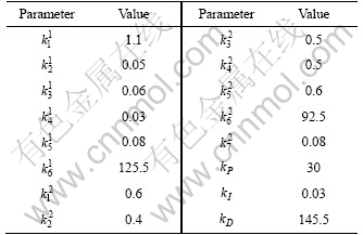
Both the controller design parameters are displayed in Table 3.
The environmental current disturbances are considered to validate the performance of bottom- following controller for the AUV.
The velocity of the current is set as

Table1 Model parameters of AUV
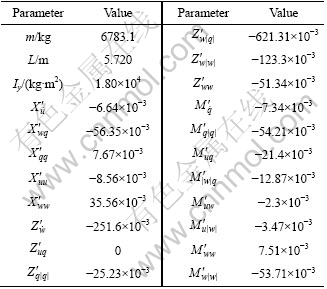
Table 2 Actuators parameters of AUV
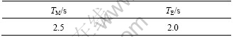
Fig. 3 Trajectories described by AUV with INSM and PID control method
Table 3 Controller parameters
And the flowing direction of the currents is 0�� (joint angle about the negative direction of x-axis). The initial forward speed of the AUV is u=0 m/s, and the desired surge speed ud is set to be 2 m/s. The initial position and attitude angle of the vehicle is chosen as (x, y, z)=(0, 0, 50) and (��, ��, f)=(0��, 0��, 0��), respectively.
Under the designed control law Eqs. (14), (23) and (24), simulation curves are shown in Figs. 4-8.
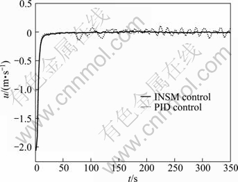
Fig. 4 Surge speed error of AUV with INSM and PID control method
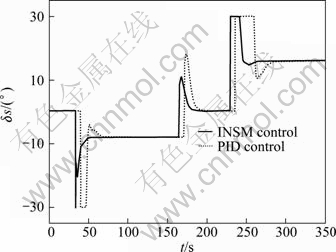
Fig. 5 Rudder angle of AUV with INSM and PID control method
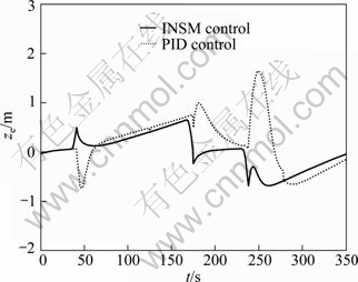
Fig. 6 Vertical bottom-following error of AUV with INSM and PID control method
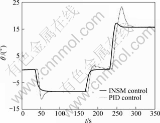
Fig. 7 Pitch angle of AUV with INSM and PID control method
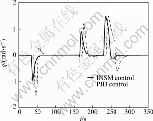
Fig. 8 Pitching rate of AUV with INSM and PID control method
It is easy to see that the INSM control approach can reduce the bottom-following error caused by the environmental current disturbances much more than the traditional PID control method. In Fig. 3, a seabed with very sharp transitions is used to evaluate the performance of the bottom-following techniques, and the control objective is to drive the AUV to track the bottom profile at a constant altitude of 10 m. The result shows that, for constant slope, the vehicle trajectory converges to the designated virtual bottom path. And the INSM control action results in a smoother path trajectory, largely reducing overshoots and the convergence time. It is also clear that, with INSM, the smoother trajectory illuminates the invariability and robustness of the proposed controller.
Since measurements of the position are often corrupted by noise, to overcome the shortcomings resulted from numerical differential action, nonlinear sliding surfaces and integral actions are added to the controller. An observer based output-feedback controller will be studied further. The capabilities of the iterated sliding mode design will be exploited in underactuated AUV stabilization. Future works also include controller parameters optimizing.
6 Conclusions
1) For the bottom-following problem of underactuated AUVs, a nonlinear decoupling control method is designed to drive the AUV to track the desired bottom profile.
2) The vertical bottom-following error and pitch angle error are stabilized by means of the rudder alone, and the longitudinal bottom-following error and forward speed can be adjusted by the thruster.
3) Furthermore, the reference course generated by an accurate model is not needed. The practicality lies in that the complex and unnecessary estimation of system uncertainties and environmental disturbances is left out. Simulation results successfully demonstrate the capability of the proposed control strategy.
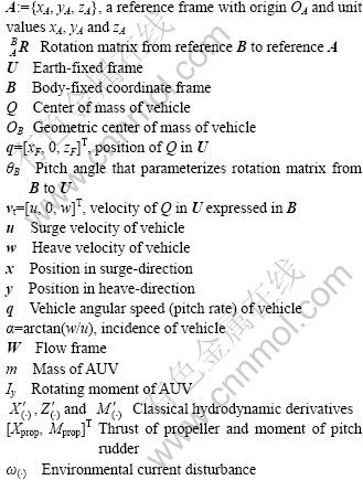
Nomenclature
References
[1] CACCIA M, BONO R, BRUZZONE G. Variable-configuration UUVs for marine science applications [J]. IEEE Robotics and Automation Magazine, 1999, 6(2): 22-32.
[2] BONO R, CACCIA M, VERUGGIO G. Simulation and control of an unmanned underwater vehicle [C]// IEEE International Conference on Robotics and Automation. Nagoya, Japan, 1995: 1573-1578.
[3] SANTOS S, SIMON D, RIGAUD V. Sensor-based control of a class of underactuated autonomous underwater vehicles [C]// Proceedings of the 3th IFAC Workshop on Control Applications in Marine Systems. Norway: IEEE, 1995: 107-114.
[4] ZAPATA R, LEPINAY P. Collision avoidance and bottom following of a torpedo-like AUV [C]// Oceans Conference Record. Fort Lauderdale, USA: IEEE, 1996: 571-575.
[5] GAO Jian, XU De-min, ZHAO Ning-ning, YAN Wei-sheng. A potential field method for bottom navigation of autonomous underwater vehicles [C]// Proceedings of the 7th World Congress on Intelligent Control and Automation. Chongqing: IEEE, 2008: 25-27.
[6] SMITH, SAMUEL M, WHITE K, XU Min. Fuzzy logic flight and bottom following controllers for the ocean voyager II AUV [C]// Proceedings of the Joint Conference on Information Sciences. Pinehurst, USA: IEEE, 1994: 56-59.
[7] BENNETT A, LEONARD J, BELLINGHAM G. Bottom following for survey-class autonomous underwater vehicles [C]// Proceedings of the 9th Int Symp on Unmanned Untethered Submersible Technology. Durham: IEEE, 1995: 327-336.
[8] CACCIA M, VERUGGIO G. Active sonar-based bottom-following for unmanned underwater vehicles [J]. Control Engineering Practice, 1999, 7(4): 459-468.
[9] WANG S, ZHANG H, HOU W. Control and navigation of the variable buoyancy AUV for underwater landing and take off [J]. International Journal of Control, 2007, 80(7): 1018-1026.
[10] CARLOS S, RITA C, NUNO P, ANT?NIO P. A bottom-following preview controller for autonomous underwater vehicles [J]. IEEE Transactions on Control Systems Technology, 2009, 17(2): 257-266.
[11] LIONEL L, DIDLIK S. Nonlinear path-following control of an AUV [J]. Ocean Engineering, 2007, 34(11): 734-1744.
[12] LI Ji-hong, PAN L. A neural network adaptive controller design for free-pitch-angle diving behavior of an autonomous underwater vehicle [J]. Robotics and Autonomous Systems, 2005, 52(2/3): 132-147.
[13] LI Ye, PANG Yong-jie, WAN Lei. A fuzzy motion control of AUV based on apery intelligence [C]// Chinese Control and Decision Conference. Guilin, China: IEEE, 2009: 1316-1321.
[14] ENCARNACAO P, PACOAH A, ARCAK M. Path following for autonomous marine craft [C]// Proceedings of the 5th IFAC on MCMC. Copenhagen, Denmark: IEEE, 2000: 27-29.
[15] MICHELE A, GIUSEPPE C and GIOVANNI I. A planar path following controller for underactuated marine vehicles [C]// IEEE Conference on Control and Automation. Dubrovnik: IEEE, 2001: 27-29.
[16] BU Ren-xiang, LIU Zheng-jiang. Path following and stabilization of underactuated surface ships [C]// Chinese Control and Decision Conference. Guilin, China: IEEE, 2009: 262-267.
[17]
[18] MUGDHA N, SAHJENDRA N. State-dependent Riccati equation-based robust dive plane control of AUV with control constraints [J]. Ocean Engineering, 2007, 34(11): 1711-1723.
[19] ENCARNACAO P, PASCOAL A. 3D Path following for autonomous underwater vehicles [C]// Proceedings of the 39th Conference on Decision and Control. Sysdney, Australia: IEEE, 2000: 2977-2982.
[20] BU Ren-xiang. Nonlinear feedback control of underactuated surface ships [D]. Dalian: Dalian Maritime University, 2008. (in Chinese).
[21] SLOTINE E, LI W. Applied nonlinear control [M]. Englewood Cliffs, NJ: Prentice-Hall, 1991: 86-114.
[22] ASTROM J, WITTENMARK B. Adaptive control [M]. New York: Addison-Wesley, 1995: 48-56.
(Edited by YANG Bing)
Foundation item: Project(61174047) supported by the National Natural Science Foundation of China; Project(20102304110003) supported by the Doctoral Fund of Ministry of Education of China; Project(51316080301) supported by Advanced Research
Received date: 2011-03-23; Accepted date: 2011-11-18
Corresponding author: JIA He-ming, PhD; Tel: +86-13206666920; E-mail: jiaheminglucky99@126.com
Abstract: The bottom-following problem for underactuated autonomous underwater vehicles (AUV) was addressed by a new type of nonlinear decoupling control law. The vertical bottom-following error and pitch angle error are stabilized by means of the stern plane, and the thruster is left to stabilize the longitudinal bottom-following error and forward speed. In order to better meet the need of engineering applications, working characteristics of the actuators were sufficiently considered to design the proposed controller. Different from the traditional method, the methodology used to solve the problem is generated by AUV model without a reference orientation, and it deals explicitly with vehicle dynamics and the geometric characteristics of the desired tracking bottom curve. The estimation of systemic uncertainties and disturbances and the pitch velocity PE (persistent excitation) conditions are not required. The stability analysis is given by Lyapunov theorem. Simulation results of a full nonlinear hydrodynamic AUV model are provided to validate the effectiveness and robustness of the proposed controller.
