
J. Cent. South Univ. (2016) 23: 3132-3142
DOI: 10.1007/s11771-016-3379-3

Semi-empirical modeling of volumetric efficiency in engines equipped with variable valve timing system
Mostafa Ghajar, Amir Hasan KaKaee, Behrooz Mashadi
Department of Automotive Engineering, Iran university of Science and Technology, Tehran, Iran
 Central South University Press and Springer-Verlag Berlin Heidelberg 2016
Abstract:
Volumetric efficiency and air charge estimation is one of the most demanding tasks in control of today��s internal combustion engines. Specifically, using three-way catalytic converter involves strict control of the air/fuel ratio around the stoichiometric point and hence requires an accurate model for air charge estimation. However, high degrees of complexity and nonlinearity of the gas flow in the internal combustion engine make air charge estimation a challenging task. This is more obvious in engines with variable valve timing systems in which gas flow is more complex and depends on more functional variables. This results in models that are either quite empirical (such as look-up tables), not having interpretability and extrapolation capability, or physically based models which are not appropriate for onboard applications. Solving these problems, a novel semi-empirical model was proposed in this work which only needed engine speed, load, and valves timings for volumetric efficiency prediction. The accuracy and generalizability of the model is shown by its test on numerical and experimental data from three distinct engines. Normalized test errors are 0.0316, 0.0152 and 0.24 for the three engines, respectively. Also the performance and complexity of the model were compared with neural networks as typical black box models. While the complexity of the model is less than half of the complexity of neural networks, and its computational cost is approximately 0.12 of that of neural networks and its prediction capability in the considered case studies is usually more. These results show the superiority of the proposed model over conventional black box models such as neural networks in terms of accuracy, generalizability and computational cost.
Key words:
1 Introduction
Air charge estimation is one of the most demanding and challenging tasks in control of today��s internal combustion engines. It is the key element in air/fuel ratio feedforward control loop which together with the feedback control by the oxygen sensor affects the quality of torque and emission management. Furthermore using three-way catalytic converter needs a strict control of the air/fuel ratio around stoichiometric point in order to minimize exhaust pollutants [1]. Apart from the mass air flow (MAF) sensors having accuracy problems in some cases [2], there is no direct method for engine air charge measurement and hence it must be estimated based on the other engine variables. In this regard the most popular approach is speed-density equation [3] estimating the air charge flow based on its density and engine speed and volumetric efficiency. The density and engine speed can easily be estimated and measured, respectively. But the volumetric efficiency (VE) is not directly measureable. On the other hand, engine breathing is a complex phenomenon [4], and hence volumetric efficiency estimation is a challenging task and has substantial errors which in turn affects the air/fuel ratio control [5]. Specifically with introducing modern engines with various actuators such as variable valve timing (VVT) and exhaust gas recirculation (EGR) valve, VE estimation becomes even more sophisticated. All of these, and the fact that volumetric efficiency directly relates to torque generation of internal combustion engines [6], make VE estimation a challenging and attractive problem that has been under study in many researches.
Mathematical models proposed for VE estimation can be categorized into physically based models (white box), semi-empirical (gray box) models, and empirical (black box) models [7-8]. Physically based models are developed mainly based on the physical first principles such as the law of conservation of energy. ZHANG et al [9] proposed a model for VE considering variable cam timing and lift. They use an energy balance for the cylinder to investigate the main physical phenomena in gas exchange process. The result was a model with 16 regression parameters that must be tuned with experimental data. The main weakness of the model, as stated by the authors, was its low accuracy with the variations of the exhaust valve timing so that errors even up to 60% were seen. KOCHER et al [3] took a similar approach and proposed a VE model using the law of conservation of energy. The main characteristic of this model is that it has no unknown parameter in this model as all of them are calculated using physical or experimental relations and simplifying assumptions. The only problem with this model is its need to calculate the effective compression ratio from lgP-lgV diagram of the cylinder making it unsuitable for online application. In the other approach for VE modeling the cylinder air charge is modeled as a linear combination of the cylinder volume during valve events (VIVO, VIVC, VEVC, subscprits IVO represents intake valve opening timing, EVC represents exhaust valve closing timing; IVC represents intake valve closing timing) and the relevant gas (fresh air or residual gas) density. The gas density is a function of the inlet manifold pressure and the engine speed and usually is prepared as 2D look-up tables. van NIEUWSTADT et al [2] used such an approach and proposed a simple model for air charge estimation at low to medium engine speeds. An almost similar method was taken by LEROY et al [10] who proposed a model in terms of VIVC and VEVC and a term named overlap factor (OF) which must be calculated from cam lift profile and valve timings. The unknown parameters must be regressed for each load-engine speed pair and can be represented as two dimensional look-up tables as they are not smooth functions of engine speed and load.
Empirical (black box) models are developed mainly by choosing the proper regression function and hence there is no need to prior information about the physics of the system.  and
and  [11] developed a linear regression model for VE estimation at constant engine speed. The regressors were functions of input variables and were chosen based on trial and error. Many of empirical models are developed based on the universal approximators such as neural networks (NNs). They can be used for modelling any complex system with minimum prior information of the physics of the system provided that enough data are prepared for model training. Hence this type of models (especially NNs models) is suitable for modeling of complex phenomena of IC engine. They are used for modeling of engine performance and emission [12-15], maximum and indicated mean effective cylinder pressure [16-17], and volumetric efficiency [18-20]. NNs models generally need large amounts of experimental data for training and test of the model [3]. The complexity of NNs models and their weak extrapolation are the other drawbacks. Look-up tables are the other type of black box models and have been used for many years in engine management system control tasks. They also can be used for VE estimation as stated by GUZZELLA and ONDER [21]. CHAUVIN et al [22] used two dimensional look-up tables for VE prediction in terms engine speed and intake manifold pressure. Similar to NNs models, look-up tables have low extrapolation capability, need a large amount of experimental data, and do not have interpretability and generality, on the other hand they are simple and easy to use. Therefore they have a key role in engine management systems yet, specifically if the quantity is not calculable directly.
In developing of semi-empirical models both the physics of the system and experimental data are used. In this regard many of the aforementioned models are semi-empirical since both the prior knowledge about the system and experimental data are needed for their development. Some of them are close to empirical models (such as Ref. [22]), and some others (such as Ref. [9]) are close to physically based models.
As stated before, VE modeling is a challenging task due to the inherent nonlinearity and complexity of the engine gas flow phenomena. Therefore VE models usually suffer from lack of accuracy in some regions, lack of interpretability and generality, inaccurate extrapolation, or need to a large amount of data for model development. On the other hand the accuracy of VE model affects directly on the quality of performance and emission control of the engine. On the way to solve some of these problems, a semi-empirical volumetric efficiency model is proposed in this work having enough accuracy and generality, and needing very few samples of data for model development. Furthermore, the generality of the model is shown by its application for predicting of volumetric efficiency in 3 distinct types of SI engine.
2 Data generation
Model development phase in this work requires a large amount of data at extensive working range of the IC engine. The prevalent method for data generation, i.e. using engine dynamometer tests can be expensive and time consuming, especially if the required data are difficult to measure. Therefore in this work a detailed dimensional model of an engine (named here as engine No. 1), developed in GT POWER, USA, is used for data generation. The results of the validation of this numerical model with experimental data are shown in Fig. 1. As can be seen, the experimental and numerical data are consistent with each other except at 2500 r/min. This is believed to happen because of the simplified intake manifold geometry used in GT POWER numerical model.
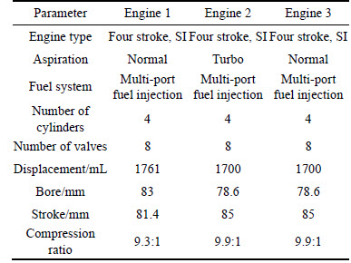
After developing the model, its performance will be tested in three cases: in the first case, the numerical data of the GT POWER model of engine No. 1 are used. The second case uses the numerical data from a detailed GT POWER model of a turbocharged engine (referred here as engine No. 2). And the third case contains the experimental data collected form dynamometer tests of engine No. 2 but without turbocharger (referred here as engine No. 3). The specifications of the three engines have been shown in Table 1.
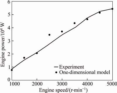
Fig. 1 Comparison of results of one dimensional model with experimental tests for engine No. 1 under wide open throttle (WOT) condition
Table 1 Specifications of engines
3 Model development
Engine volumetric efficiency is a quantity relating directly to the engine gas flow in the manifolds, ports and runners. This flow is a complex phenomenon affected by inertial effects and pressure waves. Hence its prediction requires detailed numerical models which are not proper for onboard applications. Here, in order to eliminate the intrinsic complexity of the involved thermodynamics and gas dynamics relations, a different approach is taken. This approach is based on the fact that the principle causes affecting the VE are valves timing, engine load and speed. Other quantities and phenomena (such as gas inertial effect, and engine wall heat transfer) are just intermediate causes and affected themselves by the mentioned principle causes (see Fig. 2). So from a novel point of view, these intermediate causes can be ignored and only the principle causes (as the model inputs), and volumetric efficiency (as the model output) are considered. Once the model was developed, regressed from experimental data and validated successfully in various engine operating conditions, it can be sure that all of the intermediate causes are implicitly considered in the model.
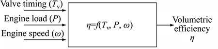
Fig. 2 Principle causes affecting volumetric efficiency
The idea proposed here is that the gas flow rate  can be related to the instantaneous cylinder volume and the amount of valve opening as follows:
 (1)
(1)
where Cd is valve flow discharge coefficient; L is valve lift; v is cylinder volume; and �� stands for instantaneous crank angle. The term CdL(��) indicates compliance of the valves against the flow and v is a measure of the flow acceptance from the cylinder. Hence the total amount of gas mass entered to the cylinder is proportional to the integral of the mentioned expression:
 (2)
(2)
The intake process of the cylinder can be divided into three phases as shown in Fig. 3. In the first phase both the intake and exhaust valves are open, and based on the pressure of the intake and exhaust manifolds, there may be a gas flow from the intake to the exhaust manifold or vice versa. In the second phase, the main amount of intake air charge enters the cylinder. The third phase is approximately between bottom dead center (BDC) and intake valve closing (IVC) timing. Accordingly the integral in Eq. (2) can be divided into three integrals:


 (3)
(3)
where A, B, C and D are constants, and ��* relates to the point of intersection of the intake and exhaust valves. Calculation of the first integral is done using LEROY and CHAUVIN��s work [23]. The lower and upper limits of the integral are shown in Fig. 4.
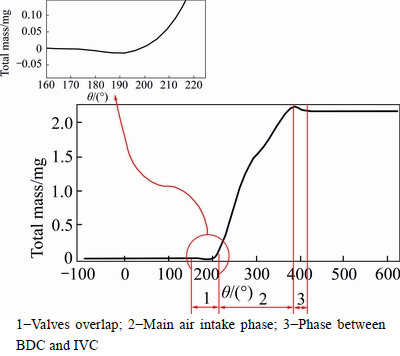
Fig. 3 Division of air intake process into three phases:
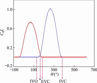
Fig. 4 Upper and lower limits of integrals in Eq. (3) (Note: Time of quantity CdL is equal for intake and exhaust valves)
As can be seen in the overlap phase, the valve with the minimum amount of CdL is determinant as it restricts the gas flow. For examining the accuracy of Eq. (3), a set of 49 data samples at various valves timings is prepared by the numerical model of engine No. 1. Then the results of air charge are used for calculating the regression parameters A, B, C and D by least square method. The results of air charge prediction are shown in Fig. 5. As can be seen, the model has good prediction capability and the normalized root mean square error (root mean square error divided by the mean of the quantity) is 0.0145. Hence, it can be a good candidate for engine air charge estimation.
The next step is to expand the model in a way that it only includes valves timings. To this end, the integrands in Eq. (3) must be estimated by a function (named here as surrogate function) in terms of crank angle. The surrogate function should have good prediction ability and its integration should not result in a very complicated expression in order to keep the model as simple as possible. After trying various functions, the following trigonometric function seems to be a good choice:
 (4)
(4)
It must be noted that although each of the quantities in the integrand (Cd, L and v) could be estimated separately, but taking this method and integrating results in very complicated expressions that are not acceptable as a simple and computational cost-effective model. Substituting Eq. (4) in Eq. (3) results in:


 (5)
(5)
where Ki (1��i��8) are constants. All of the input variables of this model are valves timings except ��* which is the crank angle in which the terms CdL for the intake and exhaust manifolds have the same values. As proved in Appendix A, by assuming the first order Taylor approximation, it can be shown that the variations of ��* linearly relates to the variations of IVO time, TIVO and EVC time, TEVC. This means that ��* itself linearly relates to TIVO and TEVC:
 (6)
(6)
Substituting Eq. (6) into Eq. (5) and integrating results in:


 (7)
(7)
Eliminating the terms that do not have positive effect on the prediction results in a simpler model:


 (8)
(8)
This model can predict the total inlet mass flowing to the cylinder during intake process at constant engine speed and load in terms of valves timings. Since the engine speed is constant in this stage, this model can also be used for VE calculation:

(9)
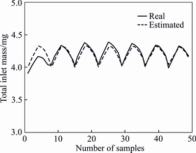
Fig. 5 Results of usage of Eq. (3) for air charge estimation with normalized root mean square error of 0.0145
3.1 Including engine speed
Engine speed directly affects the engine air charge and volumetric efficiency. This effect is so complicated that it is usually preferred to represent the model coefficients as a look-up table in terms of engine speed [2, 10]. In this work all of the constant coefficients in Eq. (9) are assumed as functions of engine speed. In other words:


 (10)
(10)
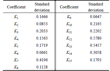
It must be noted that if all of the coefficients are considered as functions of the engine speed, the model will become very complex. The coefficient Ki of the Eq. (10) has been calculated for several engine speeds as shown in Fig. 6. As can be seen, many of these coefficients are almost constant and there is no need to be considered as functions of engine speed. For more investigation, the standard deviations of these coefficients have been calculated and represented in Table 2. Here, only the coefficients K7, K12, K13 and K14 are considered as functions of engine speed. Investigations show that all of the mentioned coefficients can be estimated with second order fractional functions:
 (11)
(11)
where Ki (1��i��20 except 7, 12, 13, 14) are constants.
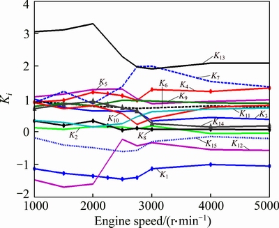
Fig. 6 Variations of coefficient Ki with engine speed
Table 2 Standard deviation of variations of coefficient Ki with engine speed
3.2 Including engine load
Engine load, often estimated by the intake manifold pressure, is the other influencing parameter for volumetric efficiency and hence must be included in the model. Here, the usual approach that assumes the coefficients of Eq. (11) vary with engine load is not considered, because it usually results in more complexity. Instead, it is assumed that the effect of the engine load is separable form the effects of other parameters. In other words:
 (12)
(12)
where p denotes intake manifold pressure. If this assumption is correct, the following relation will merely be a function of pressure for different sets of TIVO, TIVC, TEVC and ��.
 (13)
(13)
The results of an initial investigation for various values of TIVO, TIVC, and TEVC and �� are shown in Fig. 7. As can be seen, the mentioned relation is almost a function of pressure. In other words, at a constant pressure this term has almost a unique value, assuring that the separability assumption is reasonable.

Fig. 7 Variation of  with Intake manifold pressure for different values of TIVO, TIVC, TEVC, and engine speed
On the other hand, as Fig. 7 shown, the relation between the intake manifold pressure and volumetric efficiency can be assumed linear at constant engine speed and valve timing:
 (14)
(14)
where A and B are constants. Hence the model in Eq. (11) is extended as follows to include the intake manifold pressure:

 (15)
(15)
where Ki (1��i��22 except 7, 12, 13, 14) are constants. This is the ultimate model proposed here for volumetric efficiency estimation in terms of engine speed and load, and valves timings.
4 Results and discussion
Three case studies are carried out in this section in order to represent the accuracy and generalizability of the proposed model. In the first case the proposed model is used for estimating the volumetric efficiency of the comprehensive numerical model of engine No. 1. The data in second case is collected from the numerical model of engine No. 2. In the third case the experimental data collected from dynamometer tests of engine No. 3 is used and estimated by the proposed model. Furthermore, the accuracy of the proposed model is compared with that of a typical black box model. Nowadays neural networks models are widely used in modeling [24-25], control [26-27] and diagnosis [28-30] of complex and nonlinear systems. They are universal approximators and can be used for modeling any complex system with desired accuracy provided that the network has enough complexity and proper structure. Hence neural networks are chosen here as typical black box models.
4.1 Case I
For this case three sets of data are generated by the GT POWER model of engine No. 1. In the first set the engine speed and load are constant and only the valves timings vary based on Table 3. There are 125 data samples for each engine speed from which 27 samples are used for training the model and the other 98 samples are used for testing. For each engine speed the normalized root mean square error on the training and test data are shown in Fig. 8. The results are also compared with a typical neural networks model. This network has 10 neurons and one hidden layer, uses hyperbolic tangent as activation function, and Levenberg-Marquardt as training method. This is one of the most usual neural networks configurations used for predicting of multi input single output systems. The results show the accuracy superiority of the proposed model over neural networks model both for the training and test data.
Table 3 Ranges of variations of valves timings and engine speed in first data set

In the second set of data the engine speed is also considered as a variable and varies from 1000 to 5000 r/min. This data set contains 1250 samples from which 100 samples are used for training and the remaining for testing. The results of the proposed model and neural networks model are shown in Fig. 9. Again the superiority of the proposed model over neural networks is obvious.
In the third data set, in addition to the previous variables, the engine load varies between 0% and 100%. In this case, different sets for training and test are used. As can be seen in Figs. 10 and 11 when the amount of training data is large, the performance of the proposed model deteriorates in comparison with neural networks. This may be due to the simplifying assumption of separability of the engine load from the other parameters. However, the proposed model shows better results when the number of training data reduces. This is believed to happen because the physical aspects of the are system considered in model development phase. Hence the model has better compatibility with the data in comparison with neural networks which is just a universal approximator.
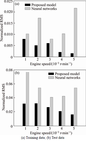
Fig. 8 Normalized RMS error in VE prediction for engine No. 1 by proposed model and neural networks (First data set):
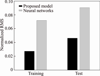
Fig. 9 Normalized RMS error in VE prediction for engine No. 1 by proposed model and neural networks (Second data set)
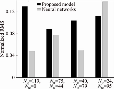
Fig. 10 Normalized RMS of training error in VE prediction for engine No. 1 by proposed model and neural networks (Third data set, training data, Ntr��number of training data; Nte�� number of test data)
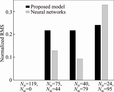
Fig. 11 Normalized RMS of test error in VE prediction for engine No. 1 by proposed model and neural networks (Third data set, test data)
4.2 Case II
In this case, the data are collected from the GT POWER model of engine No. 2 equiped with turbocharger. The main difference between the intake process in a naturally aspirated and a turbocharged engine is shown in Fig. 12. As can be seen, when both the intake and exhaust manifolds are open the gas flow in the turbocharged engine is from the intake manifold to the cylinder due to the higher pressure in the intake manifold , while in the naturally aspirated engine the gas flows form the cylinder back to the intake manifold.
The variation ranges of the variables are shown in Table 4. As can be seen in Fig. 13, the model is well capable of predicting the volumetric efficiency of the engine although it uses a turbocharger and hence its flow regime differs from a naturally aspirated engine. This shows to some extent the generalizability of the proposed model and assures its accuracy for different engines.
4.3 Case III
Another data set is provided for this case based on experimental data collected from dynamometer tests of engine No. 3. The variation ranges of the variables are shown in Table 5. For this engine, only the intake valves have been equipped with VVT system, hence only the intake valve timing varies. The results are shown in Fig. 14. As can be seen, the proposed model is well capable of predicting the experimental data, more assuring the generalizability of the model. Normalized root mean square error is 0.0152 for training data set (having 11 samples), and .0334 for test data set (having 41 samples). On the other hand the required training data set is very small. Hence it can be a good candidate for using with various engines.
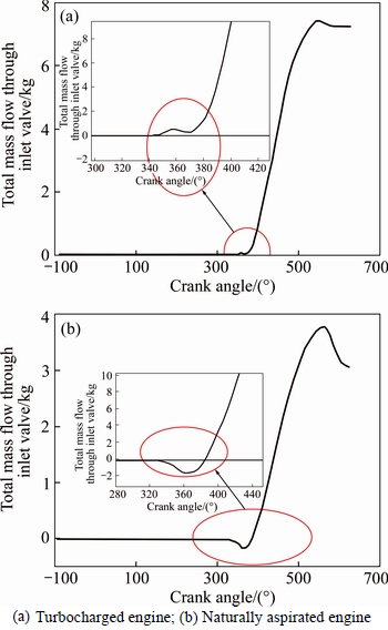
Fig. 12 Gas flow through intake valve during intake process:
Table 4 Ranges of variations of valves timings and engine speed in second case
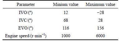
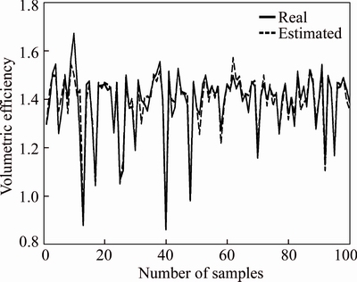
Fig. 13 Result of pridicting of volumetric efficiency of engine No. 2 equiped with turbocharger (Normalized root mean square of 0.0316, normalized maximum error of 0.1463)
Table 5 Ranges of variations of valves timings and engine speed in third case

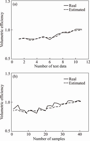
Fig. 14 Result of pridicting of volumetric efficiency of engine No. 3 (Normalized root mean square for training data of 0.0152, normalized RMS for test data of 0.0334)
4.4 Model complexity and computational cost: A comparison with neural networks
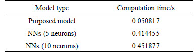
Other characteristics of the model worthy to be compared with neural networks models are its complexity and computational cost. Here the number of the coefficients of the model serves as a measure for model complexity. As can be seen in Fig. 15, the proposed model has 15, 31 and 33 coefficients in 3, 4, and 5 variable modes, respectively. On the other hand, all of the neural networks models used in this work have one hidden layer with 10 neurons. So they have 51, 61, and 71 coefficients in 3, 4 and 5 variable modes, respectively. This shows that the complexity of the proposed model is considerably less than that of neural networks. To compare computational time of the proposed model with that of the neural networks model, the both models are used for computation of the VE in 106 samples under equal conditions on a laptop with IntelCore i7-2670QM CPU and 8 GB of RAM. Results are shown in Table 6. It can be seen that the proposed model has considerably less computational time in comparison with neural networks, even if the number of neurons is reduced to 5.
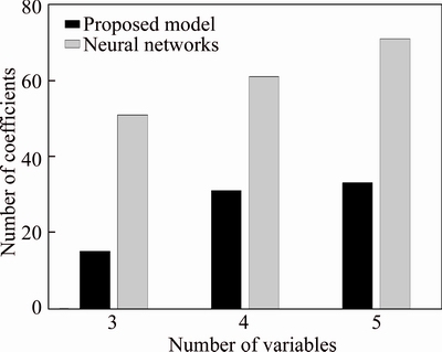
Fig. 15 A comparison between number of model coefficients of proposed model and neural networks model
Table 6 Computational cost of models in calculating of 106 data samples
It is generally believed that when the complexity of the model increases, its accuracy increases for the training data set and decreases for the test data set. But as shown, the proposed model not only has less complexity than the typical neural networks, but also its performance on the both training and test data sets is better, specifically if the number of training data samples is small. This superiority is due to the inherent difference between the two models: the proposed model has been developed based on the physics of the problem, while the neural networks model is just a universal approximator.
5 Conclusions
In this work, a novel semi-empirical volumetric efficiency model is developed based on the physics of the system and analysing the measured data. The input variables are valve timings, and engine speed and load, in the engine flow process. The following conclusions can be derived from this work.
1) After model development, its accuracy and generalizability are shown on the numerical and experimental data corresponding to the extensive working ranges of 3 distinct engines. Normalized test errors are 0.0316, 0.0152 and 0.24 for the three considered engines, respectively. The performance of the model is also compared with a typical neural networks model. It is shown that the performance of the model is much better than neural networks model both for the training and test data sets, specifically when the training data set is small.
2) On the other hand, the complexity and computational cost of the proposed model is much lower (approximately with half complexity and one tenth computational time in comparison with neural networks).
Since the model contains the major variables affecting the volumetric efficiency, it can be used for various VVT strategies such as (intake VVT, exhaust VVT and dual VVT). Furthermore, unlike physically based models, the model does not require any sensor (except the prevalent engine speed and manifold pressure sensors), or calculation of specific quantities.Hence, it can be a good candidate for onboard automotive applications in order to calculate the volumetric efficiency in an accurate and reliable manner.
3) At last, it must be noted that the proposed model does not consider the properties of the intake air (such as air pressure, temperature and humidity). Since these quantities directly affect the volumetric efficiency, in the next work the proposed model will be modified to include them.
Nomenclature
ABDC After bottom dead centre
ATDC After top dead centre
BDC Bottom dead centre
Cd Flow discharge coefficient
EGR Exhaust gas recirculation
EVC Exhaust valve closing timing (��)
EVO Exhaust valve opening timing (��)
IC Internal combustion
IVC Intake valve closing timing (��)
IVO Intake valve opening timing (��)
L Valve lift
m Intake mass flow (kg��s-1)
NN Neural networks
OF Overlap factor
RMS Root mean square
TDC Top dead centre
v Cylinder volume (m3)
VE Volumetric efficiency
VVT Variable valve timing
�� Engine speed (r/min)
�� Volumetric efficiency
�� Instantaneous crank angle, throttle angle
(��)
Appendix
Proof of Eq. (6). By assuming the first order Taylor approximation, it can be shown that ��* linearly relates to IVO and EVC. The curves of the intake and exhaust valve lifts are shown in Fig. A1 and named f(x) and g(x), respectively. The length of the point of intersection is named as ��*. If f(x) is longitudinally transferred with a value of ��, the length of the point of intersection of the two curves will be x2=��2*. Now from the point with the length x2=��2*, a horizontal line is drawn to intersect with f(x) in a point with the length of x1.
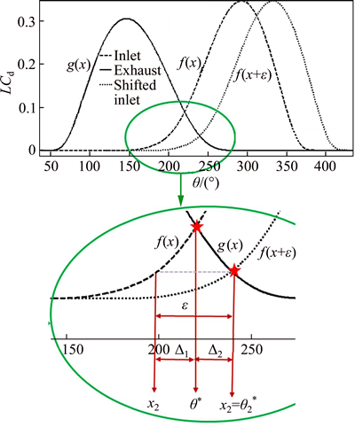
Fig. A1 Variation of point ��* with displacing of valves lift curves
Now the following relations can be derived:


 (A1)
(A1)

and

 (A2)
(A2)
Since x*=��* is a fixed point, the denominator of the right expression in Eq. (A2) is constant. In other words:
 (A3)
(A3)
where K is a constant. This means that the displacement of the point of intersection of the two curves has linear relationship with the displacement of the curves (provided that the first order Taylor approximation is used). Hence:
 (A4)
(A4)
where K1, K2 and K3 are constants.
References
[1] JANKOVIC M, MAGNER S W. Cylinder air-charge estimation for advanced intake valve operation in variable cam timing engines [J]. JSAE Review, 2001, 22: 445-452.
[2] van NIEUWSTADT M J, KOLMANOVSKY I V, HAGHGOOIE M, HAMMOUD M. Air charge estimation in camless engines [C]// SAE paper. Detroit, USA, 2001, doi:10.4271/2001-01-0581.
[3] KOCHER L, KOEBERLEIN E, van ALSTINE D G, STRICKER K, SHAVER G. Physically based volumetric efficiency model for diesel engines utilizing variable intake valve actuation [J]. International Journal of Engine Research, 2011, 13: 169-184.
[4] MALKHEDE D, KHALANE H. Maximizing volumetric efficiency of IC engine through intake manifold tuning [C]// SAE Technical Paper. Detroit, USA, 2015, doi: 10.4271/2015-01- 1738.
[5] LEROY T, CHAUVIN J, PETIT N. Airpath control of a SI engine with variable valve timing actuators [C]// American Control Conference. Seattle, Washington, USA, 2008: 2076-2083.
[6] MASI M, GOBBATO P. Measure of the volumetric efficiency and evaporator device performance for a liquefied petroleum gas spark ignition engine [J]. Energy Conversion and Management, 2012, 60: 18-27.
[7] NELLES O. Nonlinear system identification: From classsical approaches to neural networks and fuzzy models [M]. Berlin: Springer, 2001: 15.
[8] KAKAEE A H, MASHADI B, GHAJAR M. General semiempirical engine model for control and simulation of active safety systems [J]. Arabian Journal for Science and Engineering, 2015, 40(5): 1517- 1527.
[9] ZHANG R, CHANG M, TURIN R C. Volumetric efficiency model for variable cam-phasing and variable valve lift applications [C]// SAE paper. Detroit, USA, 2008, doi:10.4271/2008-01-0995.
[10] LEROY T, ALIX G, CHAUVIN J, DUPARCHY A, le BERR F. Modeling fresh air charge and residual gas fraction on a dual independent variable valve timing SI engine [J]. SAE International Journal of Engines, 2008, 1: 627-635.
[11]  O. Modeling the effect of variable cam phasing on volumetric efficiency, scavenging and torque generation [C]// SAE paper. Detroit, USA, 2010, doi:10.4271/2010-01-1190.
[12] GOLCU M, SEKMEN Y, ERDURANLI P, SALMAN M S. Artificial neural-network based modeling of variable valve-timing in a spark-ignition engine [J]. Applied Energy, 2005, 81: 187-197.
[13] ISMAIL H M, KIAT N H, QUECK C W, GAN S. Artificial neural networks modelling of engine-out responses for a light-duty diesel engine fuelled with biodiesel blends [J]. Applied Energy, 2012, 92: 769-777.
[14] TASDEMIR S, SARITAS I, CINIVIZ M, ALLAHVERDI M. Artificial neural network and fuzzy expert system comparison for prediction of performance and emission parameters on a gasoline engine [J]. Expert Systems with Applications, 2011, 38: 13912- 13923.
[15] MARTINEZ-MORALES J D, PALACIOSB E, CARRIL G A. Modeling of internal combustion engine emissions by LOLIMOT algorithm [J]. Procedia Technology, 2012, 3: 251-258.
[16] JAKUBEK S, HAMETNER C, KEUTH N. Total least squares in fuzzy system identification: An application to an industrial engine [J]. Engineering Applications of Artificial Intelligence, 2008, 21: 1277- 1288.
[17] HAMETNER C, NEBEL M. Operating regime based dynamic engine modelling [J]. Control Engineering Practice, 2012, 20: 397-407.
[18] de NICOLAO G, ROSSI C, SCATTOLINI R, SUFFRITTI M. Identification and idle speed control of internal combustion engines [J]. Control Engineering Practice, 1999, 7: 1061-1069.
[19] el HADEF J, COLIN G, TALON V, CHAMAILLARD Y. Neural model for real-time engine volumetric efficiency estimation [C]// SAE Technical Paper. Detroit, USA, 2013, doi:10.4271/2013-24-0132.
[20] MALACZYNSKI G, MUELLER M, PFEIFFER J, CABUSH D. Replacing volumetric efficiency calibration look-up tables with artificial neural network-based algorithm for variable valve actuation [C]// SAE Technical Paper. Detroit, USA, 2010, doi:10.4271/2010-01-0158.
[21] GUZZELLA L, ONDER C H. Introduction to modeling and control of internal combustion engine systems [M]. Berlin: Springer, 2004: 36.
[22] CHAUVIN J, PETIT N, ROUCHON P, CORDE G, VIGILD C. Air path estimation on diesel HCCI engine [C]// SAE Technical Paper. Detroit, USA, 2006, doi:10.4271/2006-01-1085.
[23] LEROY T, CHAUVIN J. Control-oriented aspirated masses model for variable-valve-actuation engines [J]. Control Engineering Practice, 2013, 21: 1744-1755.
[24] ISERMANN R, HAFNER M. Mechatronic combustion engines: From modeling to optimal control [J]. Eurpean Journal of Control, 2001, 7(2/3): 220-247.
[25] LI F, ZHANG J, OKO E, WANG M. Modelling of a post-combustion CO2 capture process using neural networks [J]. Fuel, 2015, 151: 156-163.
[26] HAFNER M, SCHULER M, NELLES O, ISERMANN R. Fast neural networks for diesel engine control design [J]. Control Engineering Practice, 2000, 8: 11-21.
[27]  . Feedforward neural network position control of a piezoelectric actuator based on a BAT search algorithm [J]. Expert Systems with Applications, 2015, 42: 5416-5423.
[28] BEN A J, SAIDI L, MOUELHI A, CHEBEL-MORELLO B, FNAIECH F. Linear feature selection and classification using PNN and SFAM neural networks for a nearly online diagnosis of bearing naturally progressing degradations [J]. Engineering Applications of Artificial Intelligence, 2015, 42: 67-81.
[29] SHARKEY A J C, CHANDROTH G O, SHARKEY N E. A multi-net system for the fault diagnosis of a diesel engine [J]. Neural Computing Applications, 2000, 9(2): 152-160.
[30] WANG H, GAO J, JIANG Z, ZHANG J. Rotating machinery fault diagnosis based on EEMD time-frequency energy and SOM nural ntwork [J]. Arabian Journal for Science and Engineering, 2014, 39(6): 5207-5217.
(Edited by FANG Jing-hua)
Received date: 2015-10-19; Accepted date: 2016-02-04
Corresponding author: Mostafa Ghajar, PhD Candidate; Tel: +98-0919-6458046; E-mail: m_ghajar@iust.ac.ir
Abstract: Volumetric efficiency and air charge estimation is one of the most demanding tasks in control of today��s internal combustion engines. Specifically, using three-way catalytic converter involves strict control of the air/fuel ratio around the stoichiometric point and hence requires an accurate model for air charge estimation. However, high degrees of complexity and nonlinearity of the gas flow in the internal combustion engine make air charge estimation a challenging task. This is more obvious in engines with variable valve timing systems in which gas flow is more complex and depends on more functional variables. This results in models that are either quite empirical (such as look-up tables), not having interpretability and extrapolation capability, or physically based models which are not appropriate for onboard applications. Solving these problems, a novel semi-empirical model was proposed in this work which only needed engine speed, load, and valves timings for volumetric efficiency prediction. The accuracy and generalizability of the model is shown by its test on numerical and experimental data from three distinct engines. Normalized test errors are 0.0316, 0.0152 and 0.24 for the three engines, respectively. Also the performance and complexity of the model were compared with neural networks as typical black box models. While the complexity of the model is less than half of the complexity of neural networks, and its computational cost is approximately 0.12 of that of neural networks and its prediction capability in the considered case studies is usually more. These results show the superiority of the proposed model over conventional black box models such as neural networks in terms of accuracy, generalizability and computational cost.
