

J. Cent. South Univ. (2019) 26: 684-694
DOI: https://doi.org/10.1007/s11771-019-4039-1

Spatiotemporal interpolation of precipitation across Xinjiang, China using space-time CoKriging
HU Dan-gui(������)1, 2, SHU Hong(���)1
1. State Key Laboratory of Information Engineering in Surveying, Mapping, and Remote Sensing, Collaborative Innovation Center of Geospatial Technology, Wuhan University, Wuhan 430079, China;
2. College of Computer Technology and Software Engineering, Wuhan Polytechnic, Wuhan 430074, China
 Central South University Press and Springer-Verlag GmbH Germany, part of Springer Nature 2019
Abstract:
In various environmental studies, geoscience variables not only have the characteristics of time and space, but also are influenced by other variables. Multivariate spatiotemporal variables can improve the accuracy of spatiotemporal estimation. Taking the monthly mean ground observation data of the period 1960�C2013 precipitation in the Xinjiang Uygur Autonomous Region, China, the spatiotemporal distribution from January to December in 2013 was respectively estimated by space-time Kriging and space-time CoKriging. Modeling spatiotemporal direct variograms and a cross variogram was a key step in space-time CoKriging. Taking the monthly mean air relative humidity of the same site at the same time as the covariates, the spatiotemporal direct variograms and the spatiotemporal cross variogram of the monthly mean precipitation for the period 1960�C2013 were modeled. The experimental results show that the space-time CoKriging reduces the mean square error by 31.46% compared with the space-time ordinary Kriging. The correlation coefficient between the estimated values and the observed values of the space-time CoKriging is 5.07% higher than the one of the space-time ordinary Kriging. Therefore, a space-time CoKriging interpolation with air humidity as a covariate improves the interpolation accuracy.
Key words:
space-time CoKriging; product-sum model; variogram; precipitation; interpolation��
Cite this article as:
HU Dan-gui, SHU Hong. Spatiotemporal interpolation of precipitation across Xinjiang, China using space-time CoKriging [J]. Journal of Central South University, 2019, 26(3): 684�C694.
DOI:https://dx.doi.org/https://doi.org/10.1007/s11771-019-4039-11 Introduction
Atmospheric precipitation is one of the important meteorological elements. The information of atmospheric precipitation is of great significance to the analysis of regional water resources, the prediction and management of drought and flood disasters and the management of the ecological environment [1, 2]. Xinjiang is located in the hinterland of Eurasia, surrounded by mountains, unique geographical features, fragile ecological environment and uneven distribution of water resources. It is a typical arid and semi-arid area [1]. Fully understanding the characteristics, changes and effects of precipitation resources in Xinjiang has an important role and significance to the sustainable utilization of water resources in Xinjiang and the development of a benign ecological environment.Because of the complex terrain in Xinjiang, the stations are rarely distributed, especially are scarce in the mountainous areas where precipitation is concentrated. How to generate spatial and temporal grid precipitation based on the observed precipitation and to reflect the spatiotemporal variability of precipitation is a very important work. Geostatistics is based on the theory of regionalization variables, and variogram is taken as a tool to study the science with random and structurally natural phenomena in spatial distribution [3]. In the fields of natural science and social sciences, some variables have not only spatial characteristics, but also temporal characteristics. So we should regard the variables studied as spatiotemporal random functions [4, 5]. Space-time interpolation method has become an essential mapping method to solve spatiotemporal discrete points to continuum. Space-time Kriging is a commonly used method in space-time interpolation [6�C8]. GENTON [9], MITCHELL et al [10] have studied and tested the separable spatiotemporal covariance functions, made a deep study of their advantages and disadvantages. PORCU et al [11], MASTRANTONIO et al [12], GNEITING et al [13] proposed the nonseparable, stationary covariance function, allowing time and space interaction. IACO et al [14], CESARE et al [15], MYERS [16] applied the product-sum model to model the spatiotemporal variogram. Although they have taken into account the temporal and spatial characteristics, they were limited to univariable [17�C19].
In contrast, although the traditional multivariate statistics takes into account the multivariable, it seldom takes into account the time characteristics [20, 21]. However, in some scientific researches such as hydrology, oil, soil, agriculture and forestry, atmosphere and environmental protection, the variables studied not only have time and space characteristics, but also are influenced by other related variables in the time and space domain [22, 23]. In the study of Kriging applied to spatiotemporal multivariate, on the one hand, Kriging needs to be extended to space and time, on the other hand, the univariate Kriging needs to be extended to multivariate CoKriging. The key step to study the space-time CoKriging is to model effective multivariate spatiotemporal variograms.There is a high correlation between precipitation and relative humidity [24, 25]. So in this work, taking the monthly mean precipitation of 54 meteorological stations across Xinjiang for the period 1960�C2013 as an example, taking the monthly mean air humidity of the same site at the same time as the covariates, the spatiotemporal direct variograms and the spatiotemporal cross variograms were modeled before the space-time CoKriging interpolation. Spatiotemporal product- sum variograms were used to fit the spatiotemporal variation structure of variables, and the meteorological elements were extended from space dimension to space-time dimension. At the same time, the influence of air humidity on precipitation was considered. In the process of spatiotemporal interpolation of precipitation across Xinjiang from January to December in 2013, air humidity as a covariate, the space-time Kriging interpolation was extended to the space-time CoKriging interpolation.
2 Research region and data preprocessing
2.1 Region and data introduction
The experimental region is located in Xinjiang, China. Xinjiang monthly mean precipitation data from January 1960 to December 2013 is obtained through China Meteorological science data sharing service network. There are 54 observation stations, and the station distribution is shown in Figure 1. As there is a correlation between air relative humidity and precipitation, the relative humidity of the same site at the same time is taken as the covariable in the experiment.
2.2 Data preprocessing
It is assumed that the spatiotemporal variable satisfies the second order stationary is an important prerequisite for the construction of the spatiotemporal variogram. Spatiotemporal precipitation and air relative humidity can be considered as time series. These time series usually include periodic term, trend item and random item. Therefore, the time series of precipitation is decomposed into:
 (1)
(1)
where S(t) is a periodic term; T(t) is a trend item; R(t) is a random term; and Z(t) is a time series. The random term R(t) satisfies second order stationary, taking Aksu Station as an example. In Figure 2, the time series of the observed precipitation is decomposed into a trend term, a periodic term and a random term. In Figure 3, the time series of the observed air humidity was decomposed into a trend term, a periodic term, and a random term. It can be seen from these figures that the monthly mean precipitation and monthly mean air humidity for 54 years from January 1960 to December 2013 have obvious periodicity, which is adverse to the modeling spatiotemporal variogram. However, there is no obvious trend in the time series, so only the time periodicity is removed.
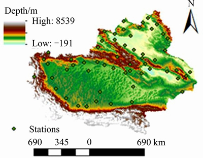
Figure 1 Study region, elevation and locations of meteorological stations
The trend term and the random term are retained. The addition model of time series decomposition is used to extract the periodic term of the variable, and the remaining residuals are used in the space-time interpolation. Autocorrelation method [26] is used to judge to stationary of residuals. As shown in Figures 4 and 5, the autocorrelation coefficient (ACF) of the time series of precipitation and relative humidity attenuates to less than 0.1 with the number of delay time. The figures show that the data is almost stationary after the removal of the periodic term.
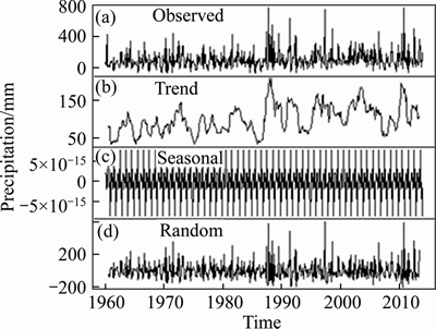
Figure 2 A comprehensive analysis of time series for precipitation at Aksu Station
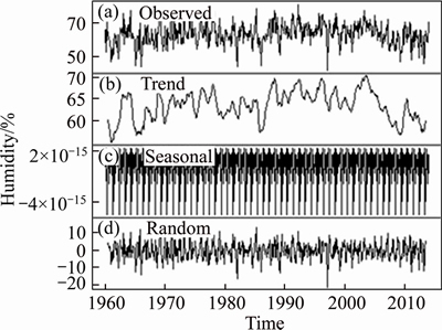
Figure 3 A comprehensive analysis of time series for air humidity at Aksu Station
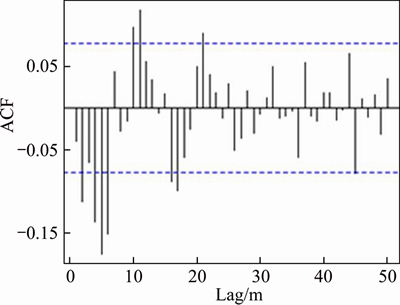
Figure 4 Autocorrelation coefficient of time series of precipitation residuals at Aksu Station
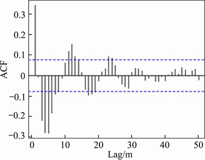
Figure 5 Autocorrelation coefficient of time series of air humidity residuals at Aksu Station
The precipitation and air humidity should also satisfy second order stationarity in space. The moving average was used to explore the trend for the residuals after the removal of the periodic term on each station. Experiments show that both precipitation and humidity are fitted with a third order polynomial which has good fitting effect.
 (2)
(2)
where Pmm is monthly mean precipitation; x and y are space coordinates; a, b, c, d, e, f and g are the coefficients obtained by the third order polynomial.
To support variograms modeling, the residuals after the removal of the periodic term and the spatial trend must be log-transformed. Before their log-transformations these residuals must undergo some preprocessing because some residuals are minus. The absolute value of the residual is log- transformed firstly. The result of the log transformation is multiplied by the absolute value of the residual, then divided by the residual, to ensure that the symbol of the residual is not changed.
 (3)
(3)
where R represents the residuals after the removal of the periodic term and the spatial trend; Lr represents the residuals after log-transformations.
3 Method
3.1 Space-time CoKriging
Space-time Cokriging (STCoKriging) is an extension of ordinary Kriging method [27]. Due to spatial and temporal correlation, the adjacent sample points in space and time are applied to the interpolation. Moreover, the best estimation method of regionalization variables is developed from univariable to multivariable, and one or more auxiliary variables are used to interpolate and estimate the interpolated variables. These auxiliary variables are related to the main variables and the correlation between the variables can be used to improve the accuracy of the interpolation. When the auxiliary information (such as air relative humidity) is easily obtained, this kind of information can be used as auxiliary factors into the STCoKriging interpolation. The air relative humidity as a covariate is conducive to the regional interpolated results. The spatiotemporal direct variograms and the spatiotemporal cross variogram of precipitation and air humidity must be used in the STCoKriging interpolation [28].
Spatiotemporal multivariate statistics is based on the theory of coregionalization variable and the tools of variogram and a study of those natural phenomena that are defined in the same temporal and spatial domain, that are statistically correlated, spatially correlated and temporal correlated. Coregionalization is a regionalized variable that has some degree of correlation in statistical sense and time series and spatial location, and it is defined in the same space and time domain. 
 is a multivariate space-time random field [26],
 (4)
(4)
where (general d��3) represents space coordinates, and
  represents time coordinates. A simple case of multiple space-time random fields is a binary space-time random field. A correlated covariate is introduced into STCoKriging to improve the interpolation accuracy. STCoKriging interpolation formula is given as:
 (5)
(5)
where is the estimated value of the precipitation at (s, t)0; Z2(s, t) is the precipitation of each station; ��2j is a set of weight coefficients of each precipitation; Z1(s, t)1i represents the air humidity of each station; ��1j is a set of weighting coefficients for each humidity; N1, N2 represent observed station number of air humidity and precipitation respectively, and N2��N1. The two Lagrange coefficients u1 and u2 are introduced and the derivation can be obtained:


 (6)
(6)
where ��11 and ��22 are the variograms of Z1 and Z2, respectively; ��12 and ��21 are the cross variograms of these two variables, ��i2(hs, ht)=��21(hs, ht). The weight coefficients (��1i, i=1, ��, N1; ��2i, j=1, ��, N2) and two Lagrange multipliers u1 and u2 can be obtained by solving the equation of linear equations formula (6). Thus, the estimated value of any station in the region can be obtained by formula (5).
3.2 Modeling of spatiotemporal direct variograms
Suppose expressed as spatiotemporal random field, where the spatiotemporal distance between two stations is h=(hs, ht), where hs represents the spatial distance of the sample, ht represents the temporal distance of the sample. When Z(s, t) satisfies the second order stationary, the covariance function can be defined [14], as follows:
 (7)
(7)
It is obvious that the covariance function is only related to the distance and is independent of the space and time site. In statistics, if the random variable expectation is unchanged, that is to say, the random variable satisfies second order spatiotemporal stationary, then the covariance matrix has a symmetric positive definiteness. In theory, the continuous function that satisfies the following requirements can be defined as an effective variogram [15]:

 (8)
(8)
where ��2 is the variance of Z(s, t). The positive definite condition is arbitrary  and arbitrary positive integer n, C must be conformed to formula (9):
 (9)
(9)
The spatiotemporal product-sum models are derived from the transformation of the pure space covariance and the pure time covariance functions by adding, multiplying, mixing, and integrating. The product-sum variograms are used to fit the spatiotemporal variation structure of spatiotemporal geographic data. Covariance function and variograms are as follows [15]:
 (10)
(10)

 (11)
(11)
where C(hs, ht) is the spatiotemporal covariance function; Cs(hs) is the spatial covariance function; Ct(ht) is the temporal covariance function. ��(hs, ht), ��s(hs), ��t(ht) are the corresponding spatiotemporal, spatial, temporal variograms, C(0, 0), Cs(0) and Ct(0) are the corresponding spatiotemporal, spatial and temporal sills. ��(0, 0)=��s(0)=��t(0)=0, conforming to k1>0, k2��0, k3��0 [29], and it is determined by formula (12).
 (12)
(12)
Assume

 and
and are respectively the sills of
  and
and . To simplify the parameters of the model, ksand kt can be considered equal to 1.
 can be further transformed into:
 (13)
(13)
 (14)
(14)
As shown in Eqs. (13) and (14), only one parameter k is determined to obtain the space-time, i.e., the product-sum variogram. The parameter k needs to satisfy the following conditions:
 (15)
(15)
Detailed derivation process and parameter estimation process are available in Ref.[29].
3.3 Modeling of spatiotemporal cross variograms
In the study of the spatiotemporal variability of variables, the key step is to determine the spatiotemporal cross variograms between variables that is used to describe the spatiotemporal continuity between the two variables. Covariance functions are defined as:

 (16)
(16)
where and
and  are the two different variables on the same site; Z1(s, t) is the mean monthly air humidity; Z2(s, t) is the mean monthly precipitation. In this case, we did not use the above definition to calculate cross variograms directly, but used the following simpler method to obtain the cross variograms indirectly [30]. Firstly, a new variable is defined:
 (17)
(17)
Add the sample values of the two variables at the same spatiotemporal site. The sum is the sample value of a new variable at the site. Then calculate the variograms of the new variable.
 (18)
(18)
The variogram of the new variable has the following relation with the direct variograms and the cross variograms of the original variables.


 (19)
(19)
Therefore, it can be obtained:
 (20)
(20)
Formula (17) shows that 
 and
and  are respectively fitted firstly in order to obtain
3.4 Post-processing
Before adding the interpolated residuals again to the estimates produced, some post-processing is needed to compensate for bias using log- transformed data. In our case, the estimates are correct for the log-transformed precipitation. Predictions made on log-transformed data from the preprocessing are back transformed using

 (21)
(21)
where P(s, t) denotes the estimates of precipitation; strend(s, t) denotes the space trend; tperiod(s, t) denotes the time periodicity;  denotes the estimates of the space-time CoKriging residuals. Correction factor is included to lower the effect of the unbiased estimates [31].
3.5 Error assessment
In order to assess the accuracy of estimation, the root mean squared error (RMSE), the bias (BIAS), mean absolute error (MAE) and Pearson��s correlation coefficient (COR) between predictions and measurements at each station are calculated using cross validation [32]. The differences between predictions and measurements are then assessed to determine the interpolation. RMSE can be used to assess the proximity of the predicted values to the observed values. The smaller the RMSE is, the smaller the bias is, the smaller the MAE is, or the higher the COR is, the higher the estimation accuracy is. The reduction of root mean square error (RRMSE) of STCoKriging relative to STOK is used to represent the degree of improvement of prediction accuracy [33].
 (22)
(22)
4 Results and analysis
4.1 Results of space-time variograms
After the time periodicity and the space trends for precipitation and air relative humidity are removed, the spatiotemporal variograms of the residuals are fitted by the product-sum model. Figure 6 shows the spatiotemporal empirical and fitted variograms of the residuals of precipitation. Figure 7 shows the spatiotemporal empirical and fitted variogram of the residuals of air humidity.
Figure 8 shows the spatiotemporal empirical and fitted variogram of the sum of the residuals of precipitation and the residuals of air humidity.
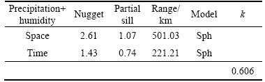
Fitted results include spatial and temporal nugget, partial sill, range and other parameters using the spatiotemporal product-sum variogram model. Tables 1�C3 respectively list the fitted results of the variograms for precipitation, air humidity, and the sum of precipitation and air humidity. The spatial and temporal variograms are all modeled by the spherical model.
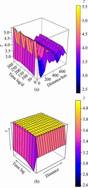
Figure 6 Spatiotemporal empirical (a) and fitted (b) variograms of precipitation residuals
After the spatiotemporal product-sum model fitting, the fitted variogram of the precipitation residuals is as follows:


 (23)
(23)
After the spatiotemporal product-sum model fitting, the fitted variogram of the air humidity residuals is as follows:


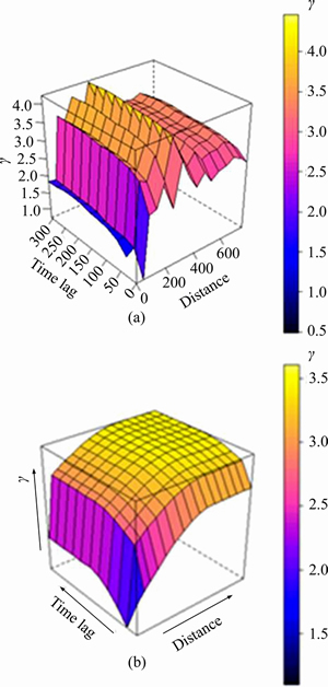
Figure 7 Spatiotemporal empirical (a) and fitted (b) variogram of air humidity residuals
 (24)
(24)
After the spatiotemporal product-sum model fitting, the fitted variogram of the new variable of precipitation residuals plus air humidity residuals is as follows:


 (25)
(25)
Therefore, according to formula (17), the spatiotemporal cross variogram of the residuals of precipitation and air humidity is as follows:
 (26)
(26)
where ��11, ��22 and ��12 in formula (26) are calculated by formula (23)�C(25), ��11 and ��22 are respectively the direct variograms of the precipitation and air humidity, ��12 is the cross variogram of the precipitation and air humidity. After ��11, ��22, ��12 are obtained, the value of lambda �� can be obtained from formula (6), so that the space-time CoKriging interpolation can be completed.
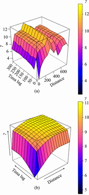
Figure 8 Spatiotemporal empirical (a) and fitted (b) variogram of sum of residuals of precipitation and residuals of air humidity
Table 1 Fitting parameters of space-time product-sum variogram for precipitation residuals
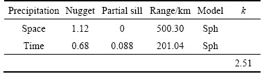
Table 2 Fitting parameters of space-time product-sum variogram for air humidity residuals
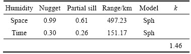
Table 3 Fitting parameters of space-time product-sum variogram for residuals of sum precipitation plus humidity
4.2 Analysis of interpolation results
The previous fitted spatiotemporal variograms are used to carry out space-time CoKriging interpolation on each station from January to December in 2013. After the interpolation results are back transformed, the temporal periodicity and the spatial trend are added, and the estimated values are obtained. The estimated results are compared with the original observation. The precipitation of each station from January to December in 2013 is interpolated by space-time CoKriging and space-time Kriging, respectively. Table 4 shows mean accuracy of 54 stations for 12 months using both interpolation methods respectively. From Table 4, we can find that RMSE, BIAS, MAE and correlation coefficient COR between the estimated value and the observed value using STCoKriging are all superior to STKriging interpolation. The space-time CoKriging interpolation reduces the mean square error by 31.46% compared with the space-time ordinary Kriging interpolation. The correlation coefficient between the estimated values and the observed values of the space-time CoKriging interpolation is 5.07% higher than the correlation coefficient of the space-time ordinary kriging interpolation. This shows that the space-time CoKriging has a better interpolation effect and the estimated values are closer to the actual measured values as a whole.
Table 4 Comparison of estimation accuracy between STCoKriging and STOKriging
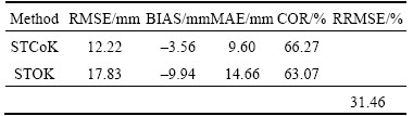
Figure 9(a) shows the error distribution of the space-time CoKriging interpolation. Figure 9(b) shows the error distribution of the space-time Kriging interpolation. Figure 9 shows the mean estimated error from January to December of 2013 each station. Each bubble represents the estimated error of the station. The larger the bubble is, the greater the error of the station. In Figure 9(a), the majority of the bubbles are smaller than ones in Figure 9(b). In Figure 9(a), it is found that the interpolation error in the Central Tianshan region of Xinjiang is the largest. The Tianshan Mountains are high altitude mountains, which are almost 1500 m above sea level. However, the observation stations of the precipitation are basically set at the lower altitude, such as at the foot of the mountain. The precipitation at the foot of the mountain is affected by more complex factors, which needs to be taken into consideration. For example, we need to increase the number of stations, set up various small scale terrain parameters and introduce them into the model, consider more complex factors in multivariate spatiotemporal interpolation methods, combine with remote sensing data, and so on. These are ways to improve interpolation accuracy.
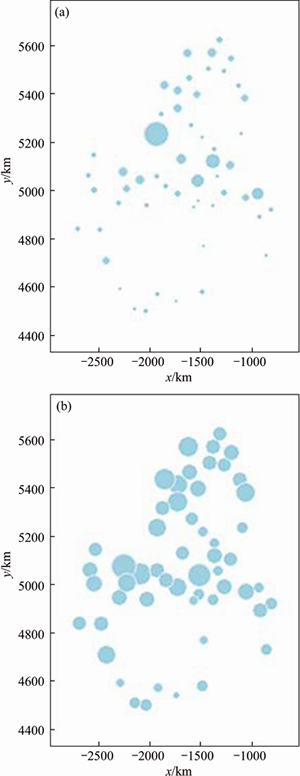
Figure 9 Error distribution of space-time CoKriging (a) and space-time Kriging (b) interpolation
5 Conclusions
The space-time CoKriging takes account of not only spatial and temporal correlation, but also the influence of auxiliary variable air relative humidity on precipitation. Space-time CoKriging makes more use of the interaction of environmental variables than the space-time Kriging of pure precipitation. The cross validation results show that the space-time CoKriging interpolation has a high accuracy and is more advantageous than the space-time ordinary Kriging interpolation. However, the correlation coefficients of estimates obtained and the observed values using these two methods are only 60%, RMSE values have more than 10 mm, showing that the interpolation accuracy is not very high, and more factors must be considered into interpolation methods. Precipitation is a complex process affected by many factors, which needs to be further studied in the future.
Spatiotemporal variograms are the foundation of the weight parameter model of space-time CoKriging interpolation. All the pure space and pure time variograms in this work use spherical models and are considered to be isotropic. The spatiotemporal product-sum model is used in the combination of time and space. There are some other methods besides the product-sum model, such as separable models, integral models and sum-metric models. In the aspect of spatiotemporal combination of variogram modeling, it is also worth further research in the future to explore a more suitable modeling method of variogram for precipitation.
References
[1] HU Dan-gui, SHU Hong, HU Hong-da, XU Jian-hui. Spatiotemporal regression Kriging to predict precipitation using time-series MODIS data [J]. Cluster Computing, 2017, 20(1): 347�C357. DOI: 10.1007/s10586- 016-0708-0.
[2] JIAPAER G, LIANG Shun-lin, YI Qiu-xiang, LIU Jin-ping. Vegetation dynamics and responses to recent climate change in Xinjiang using leaf area index as an indicator [J]. Ecological Indicators, 2015, 58: 64�C76. DOI: 10.1016/ j.ecolind.2015.05.036.
[3] YANG Yue, QIU Wen-sheng, ZENG Wei, XIE Huan, XIE Su-chao. A prediction method of rail grinding profile using non-uniform rational B-spline curves and Kriging model [J]. Journal of Central South University, 2018, 25(1): 230�C240. DOI: https://doi.org/10.1007/s11771-018-3732-9.
[4] SHU Hong. A unification of gaillangran��s spatio-temporal data models [J]. Geomatics and Information Science of Wuhan University, 2007, 32(8): 723�C726. DOI: 10.13203/ j.whugis2007.08.015. (in Chinese)
[5] KYRIAKIDIS P, JOURNEL A. Geostatistical space�Ctime models: A review [J]. Mathematical Geology, 1999, 31(6): 651�C684. DOI: 10.1023/A:1007528426688.
[6] SUBBA R T, TERDIK G, SUBBA R T, TERDIK G. A new covariance function and spatio-temporal prediction (Kriging) for a stationary spatio-temporal random process [J]. Journal of Time Series Analysis, 2017, 38(6): 936�C959. DOI: 10.1111/jtsa.12245.
[7] BAHRAMI J E, HOSSEINI S M, BAHRAMI J E, HOSSEINI S M. Predicting saltwater intrusion into aquifers in vicinity of deserts using spatio-temporal Kriging [J]. Environ Monit Assess, 2017, 189(2): 81. DOI: 10.1007/s10661-017-5795-8.
[8] RAJA N B, AYDIN O, TURKOGLU N, CICEK L. Space-time kriging of precipitation variability in Turkey for the period 1976�C2010 [J]. Theoretical and Applied Climatology, 2016, 129(1, 2): 293�C304. DOI: 10.1007/ 00704-016-1788-8.
[9] GENTON M G. Separable approximations of space-time covariance matrices [J]. Environmetrics, 2007, 18: 681�C695. DOI: 10.1002/env.854.
[10] MITCHELL M W, GUMPERTZ M G G M L. Testing for separability of space�Ctime covariances [J]. Environmetrics, 2005, 16: 819�C831. DOI: 10.1002/env.737.
[11] PORCU E P, GREGORI, MATEU J. Nonseparable stationary anisotropic space�Ctime covariance functions. Stochastic Environmental Research and Risk Assessment, 2006, 21(2): 113�C122. DOI: 10.1007/s00477-006-0048-3.
[12] MASTRANTONIO G G, JONA L, GELFAND A E, MASTRANTONIO G, LASINIO G J, GELFAND A E. Spatio-temporal circular models with non-separable covariance structure [J]. Test, 2015, 25(2): 331�C350. DOI:10.1007/s11749-015-0458-y.
[13] GNEITING T. Nonseparable, stationary covariance functions for space-time data [J]. Journal of the American Statistical Association, 2002, 97: 590�C600. DOI: 10.1198/ 016214502760047113.
[14] de IACO S, MYERS D E, POSA D. On strict positive definiteness of product and product�Csum covariance models [J]. Journal of Statistical Planning and Inference, 2011, 141(3): 1132�C1140. DOI: 10.1016/j.jspi.2010.09.014.
[15] de CESARE L, MYERS D E, POSA D. Product-sum covariance for space-time modeling: An environmental application [J]. Environmetrics, 2001, 12(1): 11�C23. DOI: 10.1002/1099-095x(200102)12:1<11::aid-env426>3.0.co;2-p.
[16] MYERS D E. Space-time correlation models and contaminant plumes [J]. Environmetrics, 2002, 13(5, 6): 535�C553. DOI: 10.1002/env.536.
[17] HEUVELINK G B M, GRIFFITH D A. Space�Ctime geostatistics for geography: A case study of radiation monitoring across parts of germany. geographical analysis [J]. 2010. 42(2): 161�C179. DOI: 10.1111/j.1538-4632.2010. 00788.x.
[18] PEBESMA E. Spacetime: Spatio-temporal data in R [J]. Journal of Statistical Software, 2012, 51(7): 1�C30. https://www.jstatsoft.org/article.
[19] XU J, SHU H. Spatio-temporal kriging based on the product-sum model: Some computational aspects [J]. Earth Science Informatics, 2014, 8(3): 639�C648. DOI: 10.1007/ s12145-014-0195-x.
[20] GAO Sheng-guo, ZHU Zhong-li, LIU Shao-min, JIN Rui, YANG Guang-chao, TAN Lei. Estimating the spatial distribution of soil moisture based on Bayesian maximum entropy method with auxiliary data from remote sensing [J]. International Journal of Applied Earth Observation and Geoinformation, 2014, 32: 54�C66. DOI: 10.1016/ j.jag.2014.03.003.
[21] KASMAEE S, RISK F M T. Reduction in Sechahun iron ore deposit by geological boundary modification using multiple indicator Kriging [J]. Journal of Central South University, 2014, 21: 2011�C2017. DOI: 10.1007/s11771-014-2150-x.
[22] KILIBARDA M, HENGL T, HEUVELINK G, GRAELER B, PEBESMA E, TADIC M P, BAJAT B. Spatio-temporal interpolation of daily temperatures for global land areas at 1km resolution [J]. Journal of Geophysical Research: Atmospheres, 2014, 119(5): 2294�C2313. DOI: 10.1002/2013JD020803.
[23] HENGL T, HEUVELINK G, TADIC M P, PEBESMA E. Spatio-temporal prediction of daily temperatures using time-series of MODIS LST images [J]. Theoretical and Applied Climatology, 2011, 107(1, 2): 265�C277. DOI: 10.1007/s00704-011-0464-2.
[24] CHEN F, ZHANG M, WANG S, QIU X, DU M. Environmental controls on stable isotopes of precipitation in Lanzhou, China: An enhanced network at city scale [J]. Sci Total Environ, 2017, 609: 1013�C1022. DOI: 10.1016/j.scitotenv.2017.07.216.
[25] JES S R, CESAR A M, ESTEBAN A G, ALBA S V, FRANCISCO N S, IBAI R, JUAN I L M. Meteorological and snow distribution data in the Izas Experimental Catchment (Spanish Pyrenees) from 2011 to 2017 [J]. Earth Syst Sci Data, 2017, 9: 993�C1005. DOI: 10.5194/essd-9- 993-2017.
[26] WANG Yan. Applied time series analysis [M]. 3rd ed. Beijing: Renmin University of China Press, 2013. (in Chinese)
[27] de IACO S, PALMA M, POSA D. Modeling and prediction of multivariate space�Ctime random fields [J]. Computational Statistics & Data Analysis, 2005, 48(3): 525�C547. DOI: 10.1016/j.csda.2004.02.011.
[28] MATEU J, PORCU E, GREGORI P. Recent advances to model anisotropic space�Ctime data [J]. Statistical Methods and Applications, 2007, 17(2): 209�C223. DOI: 10.1007/ s10260-007-0056-6.
[29] CESARE L D, MYERS D E, POSA D. Estimating and modeling space�Ctime correlation structures [J]. Statistics & Probability Letters, 2001, 51(1): 9�C14. https://www. sciencedirect.com/search/advanced?docId=10.1016/S0167-7152(00)00131-0.
[30] MYERS D E. Matrix formulation of Co-Kriging [J]. Mathematical Geology, 1982, 14(3): 249�C257. DOI: 10.1007/BF01032887.
[31] DENBY B, SCHAAP M, SEGERS A, BUILTJES P, HOR LEK J. Comparison of two data assimilation methods for assessing PM10 exceedances on the European scale [J]. Atmospheric Environment, 2008, 42(30): 7122�C7134. DOI: 10.1016/j.atmosenv.2008.05.058.
[32] KEARNS M, RON D. Algorithmic stability and sanity-check bounds for leave-one-out cross-validation [J]. Neural Computation, 1999, 11(6): 1427�C1453. DOI: 10.1162/089976699300016304.
[33] MEHDIZADEH S, BEHMANESH J, KHALILI K. A comparison of monthly precipitation point estimates at 6 locations in Iran using integration of soft computing methods and GARCH time series model [J]. Journal of Hydrology, 2017, 554: 721�C742. DOI: 10.1016/j.jhydrol.2017.09.056.
(Edited by FANG Jing-hua)
���ĵ���
����ʱ��Эͬ�����ʱ�չ����й��½���ˮ��
ժҪ���ڶԵع۲��У����о��ĵ�ѧ������������ʱ�䡢�ռ���������������������Ӱ�죬���ö�Ԫʱ��������ݣ��������ʱ�չ�ֵ�ľ��ȡ����½�����Ϊ������, ����1960��2013 ������վ�Ľ�ˮ���۲����ݵ���ƽ��ֵ, ����ʱ�տ�����ʱ��Эͬ������ֵ����, ����������2013��1 ��12�½�ˮ����ʱ�շֲ��������ʹ��ʱ��Эͬ������ֵ�����У�����ʱ��ֱ�ӱ��캯����Э���캯����ʱ��CoKriging��ֵ�Ĺؼ�һ�����Ըõ���1960��2013 ����ƽ����ˮ��Ϊ������������ͬʱ��ͬλ�õ���ƽ���������ʪ����ΪЭ�������Խ�ˮ���Ϳ������ʪ�Ƚ���ʱ��ֱ�ӱ��캯����ʱ�ս���Э���캯����ģ��ʵ��������������������ʪ����ΪЭ������ʱ��Эͬ�����IJ�ֵ������ʱ����ͨ�����IJ�ֵ�����ľ�����������31.46%������������ʪ����ΪЭ������ʱ��Эͬ�����IJ�ֵ�����Ĺ���ֵ��۲�ֵ�����ϵ����ʱ����ͨ�����IJ�ֵ���������ϵ�������5.07%����ˣ��������ʪ����ΪЭ������ʱ��Эͬ������ֵ��������˲�ֵ���ȡ�
�ؼ��ʣ�ʱ��Эͬ����𣻻���ģ�ͣ����캯������ˮ������ֵ��
Foundation item: Project(17D02) supported by the Open Fund of State Laboratory of Information Engineering in Surveying, Mapping and Remote Sensing, Wuhan University, China; Project supported by the State Key Laboratory of Satellite Navigation System and Equipment Technology, China
Received date: 2018-01-23; Accepted date: 2018-10-30
Corresponding author: SHU Hong, PhD, Professor; Tel: +86-13808617909; E-mail: shu_hong@whu.edu.cn; ORCID: 0000-0003- 2108-1797
Abstract: In various environmental studies, geoscience variables not only have the characteristics of time and space, but also are influenced by other variables. Multivariate spatiotemporal variables can improve the accuracy of spatiotemporal estimation. Taking the monthly mean ground observation data of the period 1960�C2013 precipitation in the Xinjiang Uygur Autonomous Region, China, the spatiotemporal distribution from January to December in 2013 was respectively estimated by space-time Kriging and space-time CoKriging. Modeling spatiotemporal direct variograms and a cross variogram was a key step in space-time CoKriging. Taking the monthly mean air relative humidity of the same site at the same time as the covariates, the spatiotemporal direct variograms and the spatiotemporal cross variogram of the monthly mean precipitation for the period 1960�C2013 were modeled. The experimental results show that the space-time CoKriging reduces the mean square error by 31.46% compared with the space-time ordinary Kriging. The correlation coefficient between the estimated values and the observed values of the space-time CoKriging is 5.07% higher than the one of the space-time ordinary Kriging. Therefore, a space-time CoKriging interpolation with air humidity as a covariate improves the interpolation accuracy.
