

J. Cent. South Univ. (2019) 26: 1719-1734
DOI: https://doi.org/10.1007/s11771-019-4128-1

Stability analysis for nonhomogeneous slopes subjected to water drawdown
SUN Zhi-bin(��־��)1, SHU Xing(����)1, Daniel DIAS2
1 School of Automotive and Transportation Engineering, Hefei University of Technology,Hefei 230009, China;
2. Laboratory 3SR, Grenoble Alpes University, CNRS UMR5521, Grenoble F-38000, France
 Central South University Press and Springer-Verlag GmbH Germany, part of Springer Nature 2019
Abstract:
Comparing with the homogeneous slope, the nonhomogeneous slope has more significance in practice. The main purpose of the present study is to provide a preliminary idea that how the nonhomogeneity influences the stability of slopes under four different water drawdown regimes. Two typical categories of nonhomogeneity, identified as layered profile and strength increasing with depth profile, are included in the paper, and a nonhomogeneity coefficient is defined to quantify the degree of soil properties nonhomogeneity. With a modified discretization technique, the safety factors of nonhomogeneous slopes are calculated. On this basis, the variation of safety factor with the nonhomogeneity coefficient of friction angle and the water table level are investigated. In the present example, safety factor correlates linearly with friction angle nonhomogeneity coefficient from a whole view and the influences of the water table level on safety factor is basically similar with that in homogeneous condition.
Key words:
upper bound; discretization technique; non-homogeneous slope; water drawdown��
Cite this article as:
SUN Zhi-bin, SHU Xing, Daniel DIAS. Stability analysis for nonhomogeneous slopes subjected to water drawdown [J]. Journal of Central South University, 2019, 26(7): 1719-1734.
DOI:https://dx.doi.org/https://doi.org/10.1007/s11771-019-4128-11 Introduction
Slopes located nearby a reservoir are more susceptible to landslides, which entails casualties and property losses of residential areas. The risk of slope collapse will increase significantly when the slope suffering the process of water table drawdown. Sufficient knowledge of the stability condition is vital to the protection design of such a slope. In order to provide effective stability evaluation tools, scholars have proposed numerous types of method. More details can be found in the pieces of literature by MORGENSTERN [1], PINYOL et al [2], VIRATJANDR et al [3], where the analysis approaches can be grouped into three categories: the limit equilibrium, the numerical approach, and the limit analysis.
Limit equilibrium is a widely adopted approach for the analysis of slope stability with pore pressure. MORGENSTERN [1] used such a method to evaluate the capability of the slope during the rapid water drawdown, where the pore pressure was defined by the pore-pressure coefficient. With the help of the stability charts proposed by the study, engineers can figure out the slope safety factor directly. However, the limit equilibrium method didn��t cover the stress-strain relation of soils which makes the solutions derive an approximate value rather than an exact one [4].
Alternately, the numerical simulation was also employed to estimate the slope stability affected by water drawdown. LANE et al [5] utilized the finite element method to investigate the influence of the water level drop rate and the initial position of the reservoir water level on homogeneous slopes. Lately, considering the effect of water on the soil strength, PINYOL et al [2] incorporated the influences of pore pressure into the finite element method to assess the stability of slopes subjected to both rapid and slow drawdown. The numerical simulation can provide comprehensive information of slope, such as stress, strain, and displacement, rather than only the stability condition. However, such approach is puzzled by the complication and time-consuming in the modeling process and the accuracy of the calculation more depends more on the user��s experience.
Apart from the two above methods, another attractive approach is limit analysis [6-10], which is based on the plastic mechanics rigidly. Such a method includes two different approaches: the kinematic approach and the static method. The kinematic approach, which gives a true upper bound of the limit solution, is more widespread due to the more conveniences. Through the multiple reliable validations by experiments or numerical calculations, this kinematic approach has become an effective tool for slope stability assessment [11-13].
Including the effect of the pore pressure in a kinematic mechanism, the kinematic analysis can also be employed to analyze the influence of water on a slope [14-17]. As to a slope subjected to the water drawdown process, VIRATJANDR et al [3] assumed four different water drawdown processes and then gave a closed-form solution for the slope safety. The stability results were presented as stability charts, therefore, the variation of the safety factor during the drawdown process can be obtained directly without the process of iterative calculation.
The previous researches involved with the slope subjected to water drawdown were limited to the slope with uniform soil properties, i.e., the homogeneous slope, which is not always in accordance with the real case. The non- homogeneity in soil properties has a significant influence on the stability condition of slopes [18-20]. In order to offer a more general guidance to the practical engineering, it is of practical significance to extend the reservoir slope analysis to the nonhomogeneous condition. However, an insurmountable difficult will emerge in the prediction of the velocity discontinuity surface due to the requirement of normal condition when the frequently adopted log-spiral kinematic mechanism is implemented for a non-homogeneous slope.
The presented study adopts a new type of the kinematic analysis technique, so-called the discretization technique, to overcome such shortcomings. This novel technique was originally proposed by MOLLON et al [21-24] for the face stability issue of a heterogamous tunnel and then was introduced into the slope analysis by SUN et al [19], LI et al [25], QIN et al [26]. This technique is characterized by the concept of a sliding surface consisting of a series of segments rather than being a continuous log-spiral curve, which makes the normal condition easily satisfied in a nonhomogeneous case by adjusting the location of each segment.
Aiming to provide some useful descriptions about the influence of non-homogeneity on the slopes subjected to water drawdown, this paper investigates the nonhomogeneous slope stability under four different water drawdown regimes as shown in Figure 1. Case 1 corresponds to the rapid drawdown from completely submerged condition to fully drained, similarly, Case 2 expresses the rapid drawdown with the reservoir been fully drained, Case 3 denotes the slow drawdown with the water level in slope been equal to the reservoir, and Case 4 represents the slow drawdown with the water level in slope and reservoir keep a constant.
This paper is organized as follows: First, a brief introduction of the discretization mechanism and the calculation flow are presented. Later, a general method of the computation of the weight work rate is proposed to extend to the application of the discretization to the density varying condition. With the improved approach, the safety factor of two typical nonhomogeneous reservoir slopes is solved and then the influence of soil strength parameters, geometry, and water drawdown condition is analyzed. The results are supposed to give a brief characteristic that how the non- homogeneity influences the stability of the reservoir slope.
2 Pore pressure in kinematic analysis
As mentioned, this study uses the kinematic approach to the stability evaluation of soil slopes subjected to water drawdown. The concept of taking the water effect into account in the framework of kinematic analysis is on the basis of transforming the work rate of the pore pressure into those of seepage force and buoyancy force [16]. Grounding on that and using Guess theorem, the work rate of the pore pressure can be expressed as:
 (1)
(1)
where  is the volumetric strain rated defined as
  ; u denotes the pore pressure; V denotes the volume of the potential failure block; S is the surface bounding the volume V; vi corresponds to the velocity along the falling blocks at failure, and ni is a unit vector normal to the surface S.
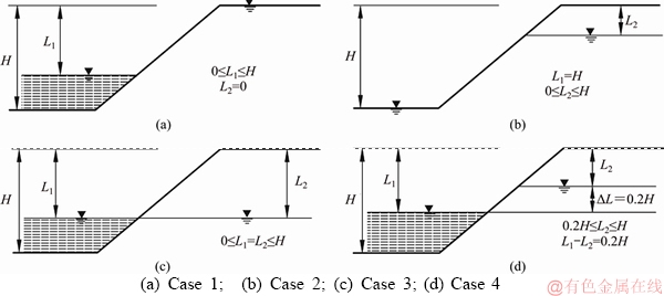
Figure 1 Four different water drawdown processes (adapted from Ref. [3]):(H: slope height; L1: vertical distance from the water level in the reservoir to the slope crest; L2: vertical distance from the water level in the slope to the slope crest)
The first integral of the right side of Eq. (1) is the work rate of pore pressure on the volumetric strain of the skeleton, and the second integral is the work rate of pore pressure on the boundary S of the structure.
Thus, when the upper bound analysis is employed, the work rate balance equation including the effect of the pore pressure can be written as:

 (2)
(2)
where ��ij and denote the stress tensor and strain rate in the admissible velocity field; Ti is the external load on the surface S; Xi is the internal force inside the area V.
Equation (2) is a complete form of the upper bound theorem under the action of pore pressure. With the equality of the work rates on the left and right sides in an admissible velocity field, the final limit state can be obtained and then the upper bound solution can be determined after an optimization process. The following analysis is based on this principle.
3 Discretization collapse mechanism generation
A suitable failure mechanism was necessary for the upper bound kinematic analysis to define a reliable admissible velocity field. The failure surface of a log-spiral shape was dominant in the conventional kinematic analysis, however, such a surface had limitations in analyzing slopes with various soil properties. Considering the need for non-homogeneous slope analysis, we adopt the discretization technique to generate the slope potential collapse surface herein. And the main principle for the generation of this mechanism will be presented in this section.
Figure 2 illustrates a reservoir slope with a discretization mechanism, where H and �� define the height and angle of the slope. It is assumed that sliding surface AC passes through the slope toe and can be identified by two parameters, r0 and ��0, where r0 is the length of OC and ��0 is the angle between the x-axis direction and the line OC. The rigid sliding block ABC, rotating around the point O with an angular velocity ��, is postulated as a rigid body. The part below the surface AC is also rigid and unmovable.
In a discretization mechanism, the velocity discontinuity surface of the slope consists of a series of the segment PiPi+1 which is determined by the discretization points P0, P1, ��, Pi, Pi+1, ��, Pn. In order to achieve geometric consistency, the angle between two adjacent radical line OPi and OPi+1 is supposed to be the same and is denoted as �Ħ�.
The value of �Ħ� determines the accuracy of the discretization, and an adequately small value of �Ħ� makes the discretization sliding surface close to the standard log-spiral surface for a homogeneous case. According to the research of SUN et al [19], �Ħ�=0.1�� is adopted in this study, which is recommended as a great combination between accuracy and time cost.
To obtain all the location of the discretization points, a ��point to point�� technique is used in this study, which means that each point is derived from the preceding one and the distribution of all discrete points is quasi-uniform.
The key to the process is to find the recursive formula to solve the coordinates of the discretization point. Thus, two points Pi and Pi+1 are taken for an example in Figure 3 to illustrate the derivation of such formula. For simplification, a coordinate system with slope toe as the origin is established.
 and
and are two vectors starting from the point O. The angle between and the negative direction of the x-axis is ��i; ni is a unit vector that perpendicular to
 In order to satisfy the flow rule of the upper bound theorem, the angle between the tangent velocity and the real velocity is required to be the friction angles ��i. This means that the angle between the vector
  and the velocity vi of the point Pi is (��-��i).
 is the velocity vector of a point Pi, whose direction is perpendicular to the vector of and can be written as
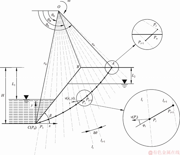
Figure 2 Discrete failure mechanism of slope
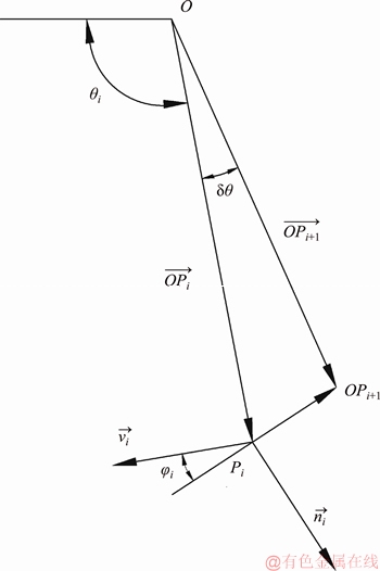
Figure 3 Illustration of generation of velocity discontinuity surface
 (3)
(3)
where �� can be set to 1.
Then decompose orthogonally to the x and y axes and can be written as
 (4)
(4)
The angle between the  and horizontal direction is
 thus the horizontal and vertical components of the vector are
 (5)
(5)
Assume where ��i is the module of and
 is a unit vector. Besides, the angle between and the horizontal direction is ��-��i, thus the horizontal and vertical components
  are
are
 (6)
(6)
is a unit vector which is perpendicular to  and the slip surface, namely
 (7)
(7)
It can be obtained by adding or subtracting vectors:
 (8)
(8)
Substituting Eq. (7) into Eq. (8) and entering the coordinate operation of the vector, the  can be expressed as
 (9)
(9)
where ��i+1 is the angle between OPi+1 and x-axis.
Then, the coordinates of the point Pi+1 can be denoted by Pi as
 (10)
(10)
where x0 and y0 are the coordinates of the rotating center O, respectively.
Starting from the point C with the recursion Eq. (10), all the discrete points on the velocity discontinuity surface can be deduced. The generation of the slip surface terminates when the ordinate yi of the point Pi is greater than (or equal to) H, then stop calculation and vector discontinuity surface is generated. Besides, if yi>H, the linear interpolation technique should be used to adjust yi, and make sure the last discrete point just fall on AB, in other words yi=H.
4 Work rate calculations
Based on the upper bound theorem of limit analysis, it is necessary to establish a virtual work rate equation as Eq. (11) to provide an upper bound solution.
W=D (11)
where W is the work rate of external forces and D is the internal energy dissipation rate. Normally, W is only defined by the work rate of soil weight W��.
However, in order to account for the effect of water in the present study, an additional work rate Wp done by pore pressure should also be included in W. The statement of the calculation of the work rates is described in more details as below.
4.1 Work rate of soil weight
This section aims to illustrate the solution process of W�� in the discretization approach. It should be noticed that a novel calculation flow is proposed here especially for soils with varying density, which is considered as an improvement to the original discretization method that only applies in the uniform density case [19].
To offer a better description, one typically layered slope with n soil layers is represented in Figure 4(a) as an example, where AC is a potential sliding surface generated by discretization technique. The dividing line between two adjacent soil layers and is denoted as ln(x), and ��n, ��n, cn are the unit weight, friction angle and cohesion of the nth layer soil, respectively.
Notice that the potential collapse block ABC is divided into a series of triangular elements by the discretization points on the sliding surface.
Thus, the total weight work rate of the whole mechanism can be achieved by the summation of all the weight work rate of each element:
 (12)
(12)
where W�� is the weight work rate of the collapse mechanism, Wi is the weight work rate of the i-th element.
To define the calculation process of Wi,Figure 4(b) describes a single triangular element BPiPi+1 with the three vertexes being B, Pi, Pi+1, respectively.
Notice that one element contains m (m��n) soil blocks which are denoted by b1, b2, ��, bk �� bm, each of them belongs to different soil layers with different unit weight. Thus, the weight work rate of the element BPiPi+1 is the sum of each block:
 (13)
(13)
where Wbk is the weight work rate of the k-th block.
The shape of the block can be a triangle or a quadrangle in one element, thus the equations of Wbk are categorized.
The weight work rate of the first triangular block BS1T1 can be expressed as
 (14)
(14)
where ��1 is the unit weight of the first layer soil, �� is the angular velocity, S1 is the area of the block BS1T1, xm is the barycentric coordinates of the block BS1T1 and x0 is the abscissa of the point O.
The general formula of weight work rate for the rest blocks can be expressed as
 (15)
(15)
where ��k is the unit weight of the m-th layer soil, Sk is the area of the triangular element BSkTk, xk is the barycentric coordinates of the triangular element BSkTk. When the subscript of changes to k-1, ��k-1,Sk-1 and xk-1 represent the corresponding index of the block k-1.
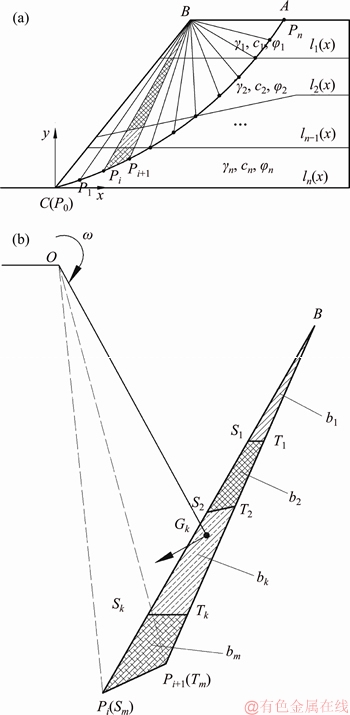
Figure 4 A layered soil slope (a) and element of failure block (b)
The expression of Sk and xk can be compiled as
 (16)
(16)
 (17)
(17)
where p is the half of the perimeter of the triangular element SBkTk; xB, xSk and xTk are the abscissa of the points B, Sk, Tk.
4.2 Work rate of pore pressure
To determine the work rate of pore pressure, the spatial distribution of pore pressure should be clarified during the process of water table drawdown. However, as pointed out by MORGENSTER [1] and VIRATJANDR et al [3], the premise of obtaining an exact solution of the pore pressure distribution only involved with, from a theoretical view, the specific hydraulic and geometry conditions with a given slope. It is difficult to obtain the generalized results for such so-called transient seepage problem.
With the purpose of achieving the pore pressure solutions with sufficient accuracy and convenience, several simplifying assumptions have been made in the pieces of literature, which are also adopted in the present study: 1) The assumption of vertical equipotential within the slope is made as shown in Figure 5; 2) Neglecting seepage, and there is no dissipation occurring after water drawdown; 3) The slope soil below the free-surface is fully saturated.
The value of the pore pressures can be expressed as
 (18)
(18)
where u is the pore pressure; hw is the vertical distance from the point to the water line; and ��w is the unit weight of water.
As shown in Figure 6, the acting surface of the pore pressure of a reservoir slope can be divided into two parts: 1) on the velocity discontinuity surface and 2) on the slope surface of the submerged area. The pore pressure in the former part is induced by the underground water in slope, while the second part is caused by the water in the reservoir.
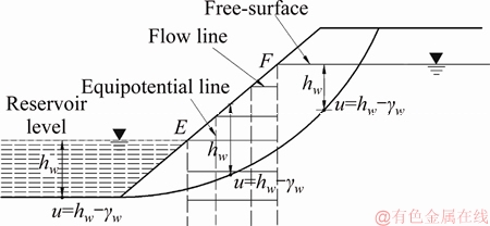
Figure 5 Details of assumption of pore pressure distribution
Accordingly, the computation of the work rate of the pore pressures is done in such parts as well.
 (19)
(19)
where Wp1 is the work rate of the pore pressure on the failure surface; Wp2 is the work rate of the pore pressure on the slope surface of the submerged area. Wp1 is related to the height of the water table in the slope and the shape of the sliding surface, namely the location of all discretization elements PiPi+1.
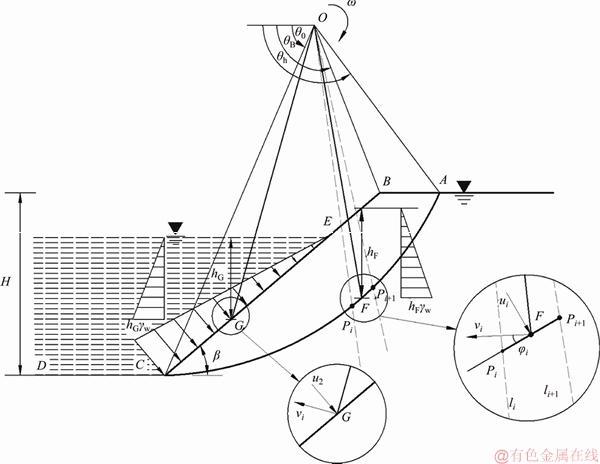
Figure 6 Details of water effect on velocity discontinuity surface and slope surface of submerged area
The expression of Wp1 can be presented as
 (20)
(20)
where u1 is the pore pressure on the element PiPi+1; vi is the velocity of the midpoint of PiPi+1; Li is the length of PiPi+1 and ��i is the friction angle of soils at the midpoint of PiPi+1.
The expressions of Li can be compiled as
 (21)
(21)
where xi and xi+1 are the x-coordinate of the point Pi and Pi+1, yi and yi+1 are the y-coordinate of the point Pi and Pi+1.
The pore pressure caused by the reservoir water acts on the surface CE, where the point C is the slope toe and the point E is the intersection between the water table and the slope surface. Thus, the work rate of the pore pressure for this part can be calculated by integration and can be presented as
 (22)
(22)
where u2 is the pore pressure to the slope surface of the submerged area; vi is the velocity of the surface and ni is the unit vector perpendicular to the surface CE.
4.3 Work dissipation rate
Owing to the rigid block assumptions mentioned in previous, the internal energy dissipation only occurs on the critical sliding surface AC. Like the computation of W��, the work dissipation rate D can be achieved by the summation of the work dissipation rate per discrete segment PiPi+1, which can be expressed as
 (23)
(23)
where ci and ��i represent the cohesion and friction angle at the midpoint of PiPi+1; Ri is the distance from O to the midpoint of PiPi+1. The expressions of Ri can be compiled as:
 (24)
(24)
5 Safety factor calculation
With the various initial values of ��0 and r0, a series of potential collapse surfaces with different safety factors can be generated. The strength reduction method is conducted to obtain the true value FS that reflects the steady state of the slope which is the minimum of these safety factors. The method is based on the idea that adopting discounted shear strength to make slope on the verge of failure, which specific details can be seen in Eq. (25).
 (25)
(25)
Therefore, the calculation of the minimum safety factory in this study is realized through the computer program, and the mathematical optimization problem is considered in the process. The specific calculation steps are shown in Figure 7.
6 Comparison and parametric analysis
6.1 Comparison of homogenous slopes with others results
In order to prove the accuracy of the discretization-based method, we calculate the safety factor of a homogeneous slope in the four water drawdown regimes mentioned in the introduction section and conduct the validation the discretization-based results with the previous achievement may be due to the two diverse assumptions of the plastic behavior of soils in different approaches: associated flow in limit analysis and non-associated flow in numerical simulation, as pointed out by VIRATJANDR et al [3]. During the validation, the stability factor c/��H of the slope is set to 0.05 and the slope inclination is 1:2.
As listed in Table 1, the comparison shows that the maximum difference between the presented results and those of VIRATJANDR et al [3] is only 4.25%, which is within a reasonable limit. The good agreement illustrates that the proposed method can give a reasonable solution to the slope stability in drawdown conditions.
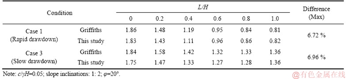
Moreover, LANE et al [5] adopted the numerical simulation to investigate the slope stability issues in two different water drawdown conditions: the rapid drawdown process and the slow drawdown process, namely the Case 1 and Case 3 in the presented paper.
To make the presented study more convincing,another validation was further carried out with the results by LANE et al [5]. It can be observed that, as shown in Table 2, the safety factors by LANE et al [5] and the present study are quite close with the maximum difference 6.9%, which indicates that the solutions derived from this present study are accurate and reasonable for the stability of slope subjected to water drawdown. The major reason of the differences in comparisons may be due to the two diverse assumptions of the plastic behavior of soils in different approaches: associated flow in limit analysis and non-associated flow in numerical simulation, as pointed out by VIRATJANDR and MICHALOWSKI [3].
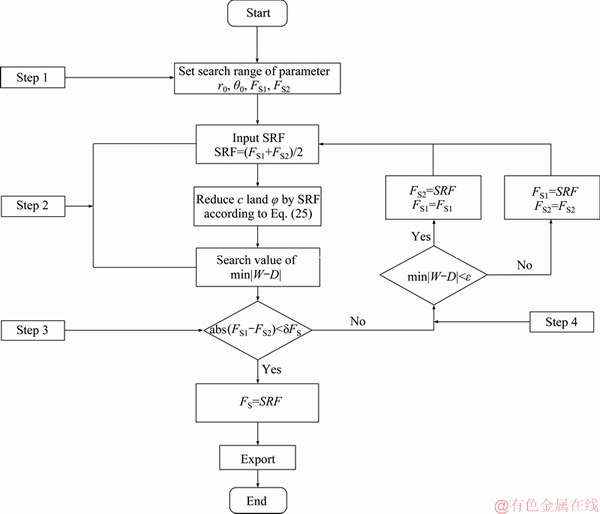
Figure 7 Computation and optimization flow of safety factor
Table 1 Comparison of safety factor with traditional kinematic analysis method
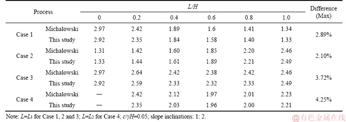
Table 2 Comparison of results with finite element method
6.2 Parametric analysis of non-uniform soil slope
Due to the complex geology and environment effect in the formation history of soils, the non- homogeneity of soil exists in various forms [18, 27]. Roughly the non-homogeneity types of slopes can be divided into two categories: the soil strength distributing linearly throughout the slope [6, 26] and the soil strength being non-uniform for different slope layers [28-30].
Practically, cohesion and friction angle can illustrate a variation in the soil space. Most previous researches were only involved with the effect of the variation of cohesion and/or friction angle.
Considering the unique merit of analyzing the friction angle varying case, and in order to especially grasp the influence of the variation of friction angle on slopes subjected to water drawdown, the focus of this paper was on the case where only the friction angle shows non- homogeneity. Moreover, for the purpose of describing the non-uniformity of slope intuitively, a parameter named the non-uniform coefficient of the friction angle ���� is introduced, which is able to quantify the degree of the non-homogeneity of friction angle of slope to a certain extent.
6.2.1 Stratified soil slope profile
To give a typical example of the layered slope, a simple two-layered soil slope is discussed as sketched in Figure 8, which has two soil layers with the same height. The geometry parameters of the slope and the detail strength parameters of soils are also presented in the figure.
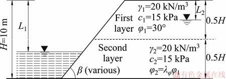
Figure 8 Schematic diagram of a two-layered soil slope under pore pressure
The friction angle of the second layer ��2 is treated as a variable with the range from 20�� to 40�� and it can be expressed by the conduct of the non-uniform coefficient of the friction angle ���� and the friction angle of the first layer ��1, namely ��2=������1. In addition, two different slope inclinations (1:2, 1:3) are considered here.
Four sets of stability charts in Figures 9-12 are plotted to provide the safety factors of the slope under rapid and slow drawdown processes. Specially, Figures 9-12 correspond to the regimes indicated in Figures 1(a)-(d), respectively, and each curve in these charts represents the change in safety factor FS with the ����. The first and second sets of stability charts (Figures 9 and 10) are given for two rapid drawdown processes, where Figure 9 (Case 1) represents a completely submerged condition to a fully drained one (L1=0). Different from Case 1, Figure 10 (Case 2) is presented for a drawdown of a slope with the reservoir has been fully drained (L1=H).
Generally, it can be found that in these two charts the variation of FS with the non-uniform coefficient ���� is roughly similar. It is indicated that Case 1 and Case 2 have the comparable stability condition under non-homogeneity in friction angle.
Comparing Figures 9(a)-12(a) with Figures 9(b)-12(b) in all charts, we can easily find that the stability of the slope decreases with the increase of slope inclination. For instance, in Figure 9, an increase of ���� from 4/6 to 8/6 leads to a 29%-34% (slope inclination 1:2) increase in the safety factor FS, while with the same variation range of ����, an increase of FS around 34%-38% is exhibited in the slope inclination 1:3 case.
Observing the variation of FS with the changing of water level in Case 1 and Case 2, two opposite patterns can be noticed.
In Case 1, as shown in Figure 9, the safety factor decreases with the increase of the water drawdown ratio L1/H. For instance, FS is decreased by around 35% (slope inclination 1:3) and 42% (slope inclination 1:2) for L1/H varying from 0 to 1.0, yet the FS increases around 37% (slope inclination 1: 3) and 40% (slope inclination 1:2) in Figure 10 (Case 2) with the same level of water drawdown.
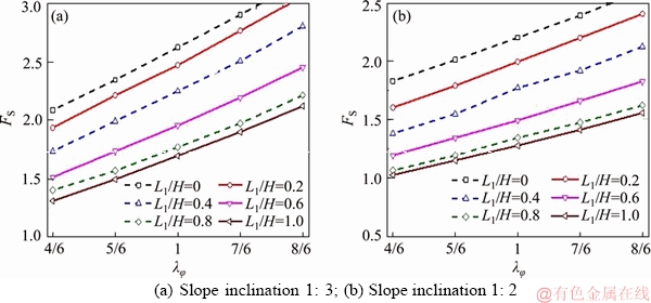
Figure 9 Safety factor for a rapid drawdown from completely submerged condition to fully drained (L2=0):
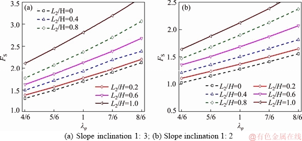
Figure 10 Safety factor for rapid drawdown with reservoir has been fully drained (L1=H):
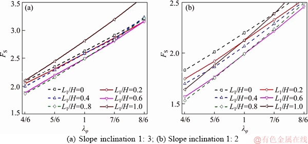
Figure 11 Slow drawdown with water level in slope is equal to reservoir (L1=L2):
This phenomenon is caused by the different effects of water in reservoir and slope on stability. Generally speaking, the pore pressure from the reservoir, which acts on the slope surface of the submerged area, is equivalent to a reverse pressure load to benefit slope stability. Thus, the water level drawdown of the reservoir in Case 1 will lead to the decline of the safety factor. Meanwhile, it is a general phenomenon that the pore pressure inside the slope is not conducive to the slope stability. Hence, the increase of L2/H in Case 2, in other words, the drawdown of the water level inside the slope, will inevitably lead to the increase of safety factor FS.
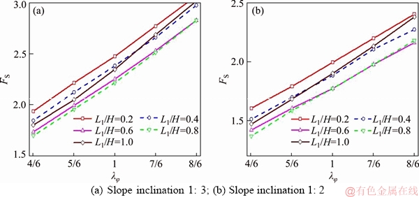
Figure 12 Safety factor for slow drawdown with water level in slope and reservoir keep a constant (L1-L2=0.2H):
Furthermore, the water level also affects the variation characteristic of FS with the non- uniformity coefficient ����. To give a whole view, the variation rate of FS and ���� decreases with the changing of the water table, no matter in Case 1 and Case 2.
The third and fourth sets of stability charts (Figures 11 and 12) are given for two slow drawdown processes, where Figure 11 (Case 3) indicates that the water level inside the slope is always equal to that in the reservoir (L1=L2), and Figure 12 (Case 4) is for the drawdown process with the water level in the reservoir and in the slope keeping constant (L1-L2=0.2H).
As shown in Figures 11 and 12, these two sets of charts have an unquestionable commonality with Case 1 and Case 2 in the variation of FS with ����. In Figure 11, FS is decreased by 27%-39% (slope inclination1:2) and 34%-41% (slope inclination 1: 3) for ���� varying from 4/6 to 8/6. In addition, in the slow drawdown process changing of safety factor with drawdown ratio L1/H has a similar regularity, but is different from the rapid drawdown case. Specifically, in Case 1 and Case 2, as L1/H increases, FS always varies monotonically, however, in Case 3 and Case 4, the varying trend of FS is not always the case. During a slow drawdown process, the value of FS has its maximum at the beginning of the drawdown process and the minimum safety factor is reached when a certain water table before the drain process is done. The characteristic of the variation of water table is consistent with the conclusions of LANE et al [5], VIRATJANDR et al [3] and GAO et al [31].
GAO et al [31] proposed the possible explanation that such phenomenon was caused by the trade-off between the work rate which done by the external pore pressure (by reservoir water benefit the stability) and the internal pore pressure (by water in slope prejudice the stability). At the beginning of water drawdown, the impact of internal pore pressure on the slope stability is greater than the external pore pressure, which leads to the reduction of the safety factor FS. However, when the water level drops to a certain extent, the external pore pressure plays a dominant role, so the safety factor FS has a small rise, ultimately.
6.2.2 Linearly increased strength profile
As shown in Figure 13, the soil friction angle is distributed linearly throughout the slope. H is the slope height, ��0 represents the friction angle on the horizontal surface passing the slope toe, the friction angle at the depth with a distance z from the slope crest can be expressed as:
 (26)
(26)
where ���� is the non-uniform coefficient of the friction angle for the case where the rate of the friction angle varies linearly with depth. The value of stability factor c/��H is 0.05 and two slope inclinations 1:2 and 1:3 are also included. In addition, the detail strength parameters of the slope are also shown in the diagram.

Figure 13 Schematic diagram of slope which friction angle varying with depth
Similar to the layered slopes, four sets of stability charts are also demonstrated in Figures 14-17 to reflect the relationship between the safety factor FS and the ���� under four special drawdown regimes.
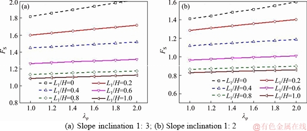
Figure 14 Safety factor for rapid drawdown from completely submerged condition to fully drained (L2=0):
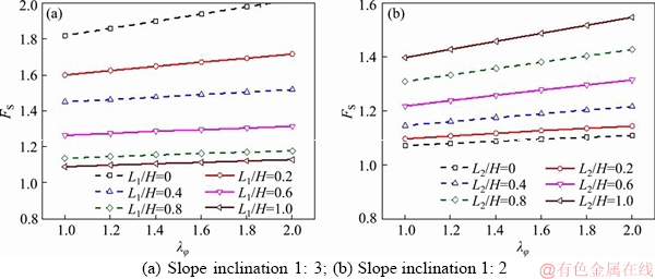
Figure 15 Safety factor for rapid drawdown with reservoir been fully drained (L1=H):
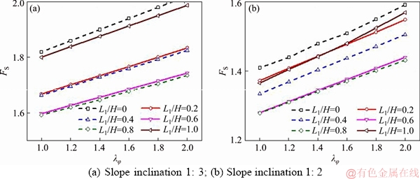
Figure 16 Slow drawdown with water level in slope equal to reservoir (L1=L2):
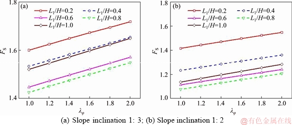
Figure 17 Safety factor for slow drawdown with water level in slope and reservoir keep a constant (L1-L2=0.2FH):
The first and second sets of stability charts (Figures 14 and 15) are for the rapid drawdown processes. Without a doubt, the increase in the non-uniform coefficient of the friction angle ���� does help to enhance the slope stability. The relationship between the non-uniform coefficient ���� and the safety factors FS is basically linear.
Observing the variation of the safety factor FS with the water drawdown ratio L1/H, there is a similarity between this case and the layered one. The safety factor FS is decreased by 40%-44% (slope inclination 1:3) and 40%-43% (slope inclination 1:2) with the water drawdown ratio L1/H varying from 0 to 1 in Figure 14. Conversely in Figure 15, variation of L1/H from 0 to 1 will increase FS by 39%-43% (slope inclination 1:3) and 39%-45% (slope inclination 1:2).
The third and fourth sets of stability charts (Figures 16 and 17) are given for slow drawdown processes, where the water in the reservoir and inside of slope always drains with equivalent rates.
It is not difficult to draw from Figures 16 and 17 that the safety factor FS exhibits a linear increase along with the coefficient of non-uniform of friction angle ����. When it turns to the influences of L1/H on the safety factor FS, the value of FS increases first and then decreases with the L1/H increase. These conclusions are consistent with the layered slope.
7 Conclusions
Based on the kinematic approach of limit analysis, the discretization technique is utilized to investigate the stability of the nonhomogeneous slopes subjected to water drawdown. The sliding surfaces of slopes are generated not with a single line but a series of non-standard curves. From the perspective of plastic theory, such a discretization failure mechanism is more reasonable.
The discretization-based results are compared with the conventional limit analysis and numerical approach as well. As expected, the present results have a good consistency with those of the two approaches, which means that the proposed mechanism is effective.
In order to better understand the influences of the non-uniformity of friction angle on slope stability, the results of the safety factor FS varying with ���� are presented in the form of stability charts. A basically linear relationship can be observed between FS and ����, of which the change rate is affected by slope inclination and water table.
During the slow drawdown process (Case 3 and Case 4), the slope safety factor is minimized when the water table reaches a certain level before drained fully. The level of the critical water table is influenced by the value of ���� when other parameters are given as constant. According to the example presented in the paper, the critical water level fluctuates between 20% and 40% of the original water level height. A preliminary conclusion can be drawn that that the critical water table for homogeneous slopes has a certain guiding significance for the nonhomogeneous slope with the variation of friction angle. However, to give a better understanding of the impact of the slope non-homogeneity on the critical water table, a more comprehensive parameter analysis will be conducted in our future research.
References
[1] MORGENSTERN N R. Charts for earth slopes during rapid drawdown [J]. G��otechnique, 1963, 13(2): 121-131.
[2] PINYOL N M, ALONSO E E, OLIVELLA S. Rapid drawdown in slopes and embankments [J]. Water Resources Research, 2008, 44(5): 303-312.
[3] VIRATJANDR C, MICHALOWSKI R L. Limit analysis of submerged slopes subjected to water drawdown [J]. Canadian Geotechnical Journal, 2006, 43(8): 802-814.
[4] CHEN J, YIN J H, LEE C F. Upper bound limit analysis of slope stability using rigid finite elements and nonlinear programming [J]. Canadian Geotechnical Journal, 2003, 40(4): 742-752.
[5] LANE P A, GRIFFITHS D V. Assessment of stability of slopes under drawdown conditions [J]. Journal of Geotechnical and Geoenvironmental Engineering, 2000, 126(5): 443-450.
[6] CHEN W F. Limit analysis and soil plasticity [M]. Amsterndam: Elsevier Scientific Pub. Co, 1975.
[7] CHEN W F, LIU X L. Limit analysis in soil mechanics [M]. New York: Elsevier, 1990.
[8] TANG Gao-peng, ZHAO Lian-heng, LI Liang, CHEN Jing-yu. Combined influence of nonlinearity and dilation on slope stability evaluated by upper-bound limit analysis [J]. Journal of Central South University, 2017, 23(7): 78-87.
[9] GAO Yu-feng, YE Mao, ZHANG Fei. Three-dimensional analysis of slopes reinforced with piles [J]. Journal of Central South University, 2015, 22(6): 2322-2327.
[10] DENG Dong-ping, LI Liang, ZHAO Lian-heng. Limit equilibrium analysis for stability of soil nailed slope and optimum design of soil nailing parameters [J]. Journal of Central South University, 2017, 24(11): 2496-2503.
[11] KUMAR J. Slope stability calculations using limit analysis [C]// Geo-Denver, 2000. Denver: American Society of Civil Engineers, 2000: 239-249.
[12] LI Zheng-wei, YANG Xiao-li. Active earth pressure for soils with tension cracks under steady unsaturated flow conditions [J]. Canadian Geotechnical Journal, 2018, 55(12): 1850-1859
[13] LI Yong-xin, YANG Xiao-li. Three-dimensional seismic displacement analysis of rock slopes based on Hoek-Brown failure criterion [J]. KSCE Journal of Civil Engineering, 2018, 22(11): 4334-4344.
[14] MILLER T W, HAMILTON J M. A new analysis procedure to explain a slope failure at the Martin Lake mine [J]. G��otechnique, 1989, 39(1): 107-123.
[15] MILLER T W, HAMILTON J M. A new analysis procedure to explain a slope failure at the Martin Lake mine [J]. G��otechnique, 1990, 40(1): 145-147.
[16] MICHALOWSKI R L. Slope stability analysis: A kinematical approach [J]. G��otechnique, 1995, 45(2): 283-293.
[17] XU Jing-shu, LI Yong-xin, YANG Xiao-li. Seismic and static 3D stability of two-stage slope considering joined influences of nonlinearity and dilatancy [J]. KSCE Journal of Civil Engineering, 2018, 22(10): 3827-3836.
[18] PAN Qiu-jing, DIAS D. Face stability analysis for a shield-driven tunnel in anisotropic and nonhomogeneous soils by the kinematical approach [J]. International Journal of Geomechanics ASCE, 2016, 16(3): 1-11.
[19] SUN Zhi-bin, LI Jian-fei, PAN Qiu-jing, DIAS D, LI Shu-qing, HOU Chao-qun. Discrete kinematic mechanism for nonhomogeneous slopes and its application [J]. International Journal of Geomechanics, 2018, 18(12), 04018171.
[20] HAN Chang-yu, CHEN Jin-jian, XIA Xiao-he, WANG Jian-hua. Three-dimensional stability analysis of anisotropic and non-homogeneous slopes using limit analysis [J]. Journal of Central South University, 2014, 21(3): 1142-1147.
[21] MOLLON G, DIAS D, SOUBRA A H. Face stability analysis of circular tunnels driven by a pressurized shield [J]. Journal of Geotechnical and Geoenvironmental Engineering, 2010, 136(1): 215-229.
[22] MOLLON G, DIAS D, SOUBRA A H. Rotational failure mechanisms for the face stability analysis of tunnels driven by a pressurized shield [J]. International Journal for Numerical and Analytical Methods in Geomechanics, 2011a, 35(12): 1363-1388.
[23] MOLLON G, PHOON K K, DIAS D, SOUBRA A H. Validation of a new 2D failure mechanism for the stability analysis of a pressurized tunnel face in a spatially varying sand [J]. Journal of Engineering Mechanics, 2010b, 137(1): 8-21.
[24] MOLLON G, DIAS D, SOUBRA A H. Continuous velocity fields for collapse and blowout of a pressurized tunnel face in purely cohesive soil [J]. International Journal for Numerical and Analytical Methods in Geomechanics, 2013, 37(13): 2061-2083.
[25] LI Tian-zheng, YANG Xiao-li. Probabilistic stability analysis of subway tunnels combining multiple failure mechanisms and response surface method [J]. International Journal of Geomechanics, 2018, 18(12): 04018167.
[26] QIN Chang-bing, CHIAN Siau-chen. Bearing capacity analysis of a saturated non-uniform soil slope with discretization-based kinematic analysis [J]. Computers and Geotechnics, 2018, 96(11): 246-257.
[27] YANG Xiao-li, ZHANG Sheng. Risk assessment model of tunnel water inrush based on improved attribute mathematical theory [J]. Journal of Central South University, 2018, 25(2): 379-391.
[28] KUMAR J, SAMUI P. Stability determination for layered soil slopes using the upper bound limit analysis [J]. Geotechnical and Geological Engineering, 2006, 24(6): 1803-1819.
[29] IBRAHIM E, SOUBRA A H, MOLLON G, RAPHAEL W, DIAS D, RAED A. Three-dimensional face stability analysis of pressurized tunnels driven in a multilayered purely frictional medium [J]. Tunnelling and Underground Space Technology, 2015, 49(6): 18-34.
[30] YANG Xiao-li, LI Zheng-wei. Comparison of factors of safety using a 3D failure mechanism with kinematic approach [J]. International Journal of Geomechanics, 2018, 18(9): 04018107
[31] GAO Yu-feng, ZHU De-sheng, ZHANG Fei, LEI G H, QIN Hong-yu. Stability analysis of three-dimensional slopes under water drawdown conditions [J]. Canadian Geotechnical Journal, 2014, 51(11): 1355-1364.
(Edited by HE Yun-bin)
���ĵ���
ˮλ�½������·Ǿ��ʱ����ȶ��Է���
ժҪ������ʱ�����ȣ��Ǿ��ʱ��¶���ʵ�ʹ����и������塣���о�������������Ǿ�����������ˮλ�½�ģʽ�¶Ա����ȶ��Ե�Ӱ�졣�ڿ��Ƿֲ���ǿ���������������������ͷǾ����ԵĻ����ϣ������˷Ǿ�����ϵ������������ǿ�ȵķǾ����Գ̶ȡ����øĽ�����ɢ���������������˲�ͬ�����·Ǿ��ʱ��µİ�ȫϵ��Fs���о���Fs��Ħ���ǷǾ���ϵ���Լ�ˮλ�߶ȵı仯���ɡ������Ͽ�Fs��Ħ���ǷǾ���ϵ����������أ���ˮλ��Fs��Ӱ������ʱ��»������ơ�
�ؼ��ʣ���������ɢ���������Ǿ��ʱ��£�ˮλ�½�
Foundation item: Project(51408180) supported by the National Natural Science Foundation of China
Received date: 2018-12-24; Accepted date: 2019-02-22
Corresponding author: SUN Zhi-bin, PhD, Associate Professor; E-mail: sunzb@hfut.edu.cn; ORCID: 0000-0002-3607-8825
Abstract: Comparing with the homogeneous slope, the nonhomogeneous slope has more significance in practice. The main purpose of the present study is to provide a preliminary idea that how the nonhomogeneity influences the stability of slopes under four different water drawdown regimes. Two typical categories of nonhomogeneity, identified as layered profile and strength increasing with depth profile, are included in the paper, and a nonhomogeneity coefficient is defined to quantify the degree of soil properties nonhomogeneity. With a modified discretization technique, the safety factors of nonhomogeneous slopes are calculated. On this basis, the variation of safety factor with the nonhomogeneity coefficient of friction angle and the water table level are investigated. In the present example, safety factor correlates linearly with friction angle nonhomogeneity coefficient from a whole view and the influences of the water table level on safety factor is basically similar with that in homogeneous condition.
