J. Cent. South Univ. Technol. (2008) 15: 552-557

DOI: 10.1007/s11771-008-0104-x

Solution to reinforcement learning problems with artificial potential field

XIE Li-juan(谢丽娟)^{1, 2}, XIE Guang-rong(谢光荣)¹, CHEN Huan-wen(陈焕文)^{2, 3}, LI Xiao-li(李小俚)⁴

(1. Institute of Mental Health, Xiangya School of Medicine, Central South University, Changsha 410011, China;

2. School of Computer and Communication, Changsha University of Science and Technology,

Changsha 410076, China;

3. Department of Computer Engineering, Hunan College of Information, Changsha 410200, China;

4. School of Computer Science, University of Birmingham, Birmingham, B15 2TT, UK)

Abstract: A novel method was designed to solve reinforcement learning problems with artificial potential field. Firstly a reinforcement learning problem was transferred to a path planning problem by using artificial potential field(APF), which was a very appropriate method to model a reinforcement learning problem. Secondly, a new APF algorithm was proposed to overcome the local minimum problem in the potential field methods with a virtual water-flow concept. The performance of this new method was tested by a gridworld problem named as key and door maze. The experimental results show that within 45 trials, good and deterministic policies are found in almost all simulations. In comparison with WIERING’s HQ-learning system which needs 20 000 trials for stable solution, the proposed new method can obtain optimal and stable policy far more quickly than HQ-learning. Therefore, the new method is simple and effective to give an optimal solution to the reinforcement learning problem.

Key words: reinforcement learning; path planning; mobile robot navigation; artificial potential field; virtual water-flow

1 Introduction

Reinforcement learning(RL) was well surveyed in Refs.[1-2]. In general, reinforcement learning has two typical methods: one is to search the space of value functions, the other is to search the space of policies, which are exemplified by a temporal difference(TD) method and an evolutionary algorithm(EA) method, respectively. So far, reinforcement learning still has many problems waiting for answer during the process of scaling up to realistic tasks, including the problems associated with very large state spaces, partially observable states, rarely occurring states and unknown environments^[1]. A potential solution to these problems is to use hierarchical decomposition methods or modular reinforcement learning systems. Often, a complicated task may be decomposed into a multiple-level hierarchy of subtasks (or subproblems, options, macro-actions), which will reduce the complexity of the target problem and therefore accelerate the learning process, then each subtask is individually learnt by using reinforcement learning, and finally a top-level policy is learnt to control the invocation and termination of these subtasks. The obtained subtask policies and value functions may be shared across hierarchical levels^[3-6]. Over the past decades, many different methods of hierarchical reinforcement learning have been developed^[7-12].

In a hierarchical reinforcement learning framework, subtasks are usually defined by invocation predicates, policy, termination predicates and pseudoreward functions. It is noted that subtasks are invoked and terminated by call-return-routine programming, so there exists a disadvantage in the hierarchical reinforcement learning, namely the task decomposition strongly depends on human’s knowledge and experiences, because a complete structure of the hierarchy and subtask modules is needed to provide. Designing the hierarchy of subtasks is very difficult, in particular in complex or uncertain environments. Moreover, the hierarchical structure and subtask modules are usually designed for a specific problem, and the agent has to irrevocably commit to them in both the learning and application processes. Therefore, it is challenging to make hierarchical structure and subtask modules adaptable or even to automate the design process of hierarchical decomposition^[13].

Considering existing problems in the reinforcement learning, it is worth exploiting an alternative method. In this work, the artificial potential field approach was developed in the reinforcement learning. This new method should belong to searching the space of policies directly in the reinforcement learning.

2 Method

2.1 Reinforcement learning model

In a standard reinforcement learning model, an agent connects the environment via perception and action, as shown in Fig.1. As for each interaction, the agent receives input, o, through a sensor, which senses the current state of the environment, denoted as s; then, the agent generates an action, a. The action changes the state of the environment, and this change inspires the reinforcer of the agent to generate a scalar reinforcement signal, r. Finally, the agent generates a new action that tends to increase the long-run sum of values of the reinforcement signal. In brief, a factored reinforcement learning model may be characterized by four distinct quantities: discrete environment states, discrete agent actions, discrete agent observations and scalar reinforcement signals received by the agent, denoted as S, A, O and R^[14]. In the reinforcement learning, the “task” or the “problem” is represented by a reward function. Given the reward function and a model of the domain 〈S, A, O〉,  the optimal policy is determined.

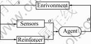
Fig.1 Standard reinforcement learning model (s denotes current state of environment; o is current observation of agent; r is reward of agent received; a is action of agent performed)

Let a policy, π, be a map from S to A, which is denoted as π: Given any policy π, a goal function or an optimal criterion is defined as

                  (1)

where  π* is the optimal policy, r(t) is the reward at time t; E( ) is the mathematical expectation; γ (0≤γ≤1) is the discount factor which ensures that the sum in Eqn.(1) is finite. The goal function is to maximize the agent’s reward over time, in other words, to find an optimal policy of the agent.

2.2 Artificial potential fields(APFs)

APF is often used as a method of path planning^[15-17]. The APF approaches are basically operated by a gradient descent search method which is directed toward minimizing the potential function. Obstacles that have to be avoided are surrounded by repulsive potential fields and the goal point is surrounded by an attractive potential field. The attractive potential is generally a bowl shaped energy well which drives a robot to its center if the environment is not obstructed. In an obstructed environment, repulsive potential energy hill is added to the attractive potential field at the locations of the obstacles. The robot experiences the force which directs to the negative gradient of the potential. This force drives the robot downhill until the robot reaches the position of the minimum energy. The attractive potential function is usually a hybrid method with parabolic and conic wells proposed by ANDREWS^[18]. The attractive potential, U_att, should increase as the robot moves away from the goal point (like potential energy increases as you move away from earth’s surface), and is described by

    ≤d   (2)

where  x represents the position vector of a robot; ρ_goal(x) (ρ_goal(x)=||x-x_goal||) represents the Euclidean distance from x to position vector of a goal x_goal; d is the radius of a quadratic range; k_a is a proportional gain of the function.

The second category of potentials, repulsive potential, is necessary to repel the robot away from obstacles which obstruct robot’s path of motion in the global attractive potential field. The following repulsive potential function, i.e. FIRAS function proposed by KHATIB^[19], is

     ≤   (3)

where  ρ₀ presents the influence distance of potential field; ρ(x) is the shortest distance from x to the position vector of obstacle x_rep, ρ(x)=||x-x_rep||; k_r is a proportional gain of the function. The distance ρ₀ depends on the maximum speed of the robot and the control period.

Thus, the global potential U(x) can be obtained by sum of the attractive potential and repulsive potential, it is

                      (4)

Potential field provides a simple and easy method for a robot to reach a goal while avoiding unknown obstacles. However, the disadvantage of this approach is that the robot often gets stuck in a local minimum of the potential, i.e. the local minimum problem will occur when the robot runs into a dead end (e.g. inside a U-shaped obstacle). The dead end can be created by a variety of different obstacle configurations, and different types of the dead ends can be distinguished. Many approaches have been proposed to find the way out from dead end for a robot, including heuristic or global recovery^[20-22], but these methods are likely to result in a non-optimal path, and a long computation time is needed. Interesting methods have also been proposed by using a global navigation function (a local minimum free potential) on a local map^[23-25]. Unfortunately, it is hard to construct a global navigation function because it has only one local minimum at the goal position x_goal.

2.3 Transmission from RL model to APF model

As can be seen in Section 2.2, APFs offer an ideal framework to model dynamical systems. Comparing a RL model with an APF model, there exist some common features for the structure. In this work, a RL model is transmitted to an APF model. The procedures are as follows.

Definition 1  A set of attractive sources, S⁺. If a reward that is received by an agent at state s is r, r∈R,  s∈Val(S) (Val( ) is a function to get value from a state set), and r＞0, then define state s as an attractive source. A set of attractive sources may be noted by S⁺={s: r=  R(s)＞0, s∈Val(S)}.

Definition 2  A set of repulsive sources, S^-. If a reward that is received by an agent at state s is r, r∈R,  s∈Val(S), and r＜0, then define state s as a repulsive source. A set of repulsive sources may be noted by S^-={s: r=R(s)＜0, s∈Val(S)}.

In terms of the two definitions, it is easy to convert a RL model to an APF model.

2.3.1 Attractive potential at current state s, U_att(s)

Let k_a be an absolute value of the reward r_att at an attractive source state s_att in Eqn.(2), denoted as |R(s_att)|, then an attractive potential at the current state s can be described by

_≤d

               (5)

where  s_att represents an attractive source state as denoted in definition 1; ρ_att(s) (ρ_att(s)=||s-s_att||) represents the Euclidean distance from state s to attractive source state s_att; d is the radius of a quadratic range. For simplifying, in this work, d is set to positive infinity, i.e. d=+∞.

2.3.2 Repulsive potential at current state s, U_rep(s)

Let k_r be an absolute value of the reward r_rep at a repulsive source state s_rep in Eqn.(3), noted by |R(s_rep)|, i.e. k_r=|R(s_rep)|, then a repulsive potential at the current state s can be described by

  (6)

where  s_rep represents a repulsive source state as denoted in definition 2; ρ_rep(s) (ρ_rep(s)=||s-s_rep||) represents the Euclidean distance from state s to the repulsive source state s_rep; ρ₀ represents the influence distance of potential field.

2.3.3 Global potential at current state s, U(s)

The global potential at state s can be obtained by sum of the attractive potential and repulsive potential, and it is described by:

U(s)=U_att(s)+U_rep(s)                           (7)

Through above transform, a reinforcement learning model becomes an artificial potential field model. The aim of the APF model is also to maximize the agent’s reward over time or to find an optimal policy, which is identical to the aim of the RL model when the discount factor γ in Eqn.(1) is set to 1. In brief, RL problems can be taken as APF problems or as path planning problems.

2.4 Virtual water flow method

In this section, a virtual water-flow method was proposed to solve the local minimum problem in APF. It is known that water flow has two characteristics: 1) flowing from high place to low place; 2) filling the place where water is unable to flow. Using the two characteristics, the basic steps of this new method are described as follows.

Step 1  Determining whether the robot locates at a local minimum or not. If U(s)＜minU(s′), and s is the current state and not a goal state, then the agent is at a local minimum. Herein, S_nei(s) presents the neighbor set of the current state s. s′∈S_nei(s) if s′ is a new state when the agent performs an action a∈Val(A) at the current state s, here A is a discrete set of agent actions as described in Section 2.1.

Step 2  Increasing the potential of local minimum state s. If the agent is at a local minimum state s, then increase the potential U(s) by

              (8)

where  v represents the speed of filling. If v≥1, Eqn.(8) is a “water filling” process, otherwise a “water releasing” process. Eqn.(8) uses the second characteristic of flowing water to overcome the local minimum problem, and the agent remembers the new adjusted U(s) for further navigation. The remember for the new adjusted potential in the agent’s navigation history makes the agent possess ability of memory and learning.

Step 3  Examining and navigating the most promising neighbors. If the current state s is not at a local minimum state, the agent will choose a neighbor of s of the lowest potential (most promising) as next state s′. Here, the first flowing water characteristic is used.

The virtual water flow method proposed here is to overcome the local minimum in normal potential field model. The method is inspired by water flow. The procedure of the method consists of 3 steps as described above. Suppose a robot navigates in an environment whose global potential has the formation of Fig.2. The robot can only move forward or backward, i.e. its action set includes 2 actions of “forward” and “backward”.

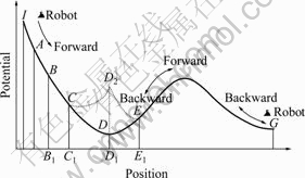
Fig.2 Local minimum problem and its solution with virtual water flow method (I, A, B, C, D, E and G represent some points in potential field.)

If the current location of the robot is C, then the value of potential isthe neighbors of C are B and D, and the potentials of them are  and  Because U(D)＜U(C)＜U(B), C is not the local minimum point. The robot moves forward from higher potential C to lower potential D directly. Now the robot is at location D. The neighbors of D are C and E. and ＜＜therefore D is a local minimum point as described by Step1. In this case, Eqn.(8) is applied to adjusting the potential of D. According to Eqn.(8), the adjusted potential of D is U(D)= D₁D₂=If v=2, then U(D)=D₁D₂=Fig.2 shows the extra potential with the dot line  In this formation of potential, the robot can escape from the local minimum point D and move to new location E because point D has higher potential than its neighbors. The process of the potential modification will go on until the robot reaches the goal position G, which is just like the water filling process in natural world.

3 Experiment and results

3.1 Experiment

The experiment involves the 25×28 maze shown in Fig.3. Stating at S, the agent has to 1) fetch a key at position K, 2) move towards the “door” (the shaded area) which normally behaves like a wall and will open (disappear) only if the agent is in possession of the key, and 3) proceed to goal G. Once the agent hits the goal, it will receive a reward of 10; if the agent hits an obstacle (the black area), it will receive a reward of -1. For all other actions there is a reward of 0. There is no additional, intermediate reward for taking the key or going through the door.

3.2 Model description

3.2.1 RL model

Environment state sets: S={S₁, S₂, S₃}, S₁ represents row of the maze; S₂ represents column of the maze; S₃ represents if the agent has key. |S|=3, Val(S₁)={1, …, 25}, Val(S₂)={1, …, 28}, Val(S₃)={0, 1}, therefore, the state space consists of 1 400 (25×28×2) states.

Agent action sets: A={A₁}, |A|=1, Val(A₁)={down, up, right, left}={1, 2, 3, 4}; agent observation sets: S=O, the model is fully observable RL.

Reward function:

3.2.2 APF model

Attractive sources: S⁺={s: r=R(s)=10}={(24, 27, 1)}, S⁺ includes 1 state as denoted in Fig.3; repulsive sources: S^-={s: r=R(s)=-1}={(1, 1, 2), (1, 2, 0), …, (25, 28, 1)}, S^- consists of 411 states, the states with key equal 204, and the states without key equal 207; attractive potential:

;

repulsive potential:

  .

where  ρ₀=3.

Speed of filling (as described in Section 2.4 and Eqn.(8)): v=2.0 in this experiment.

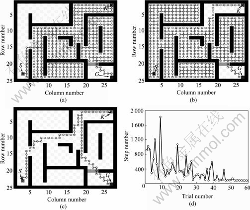
Fig.3 Path planning results using APF model for 25×28 key and door problem: (a) 1st trial, 909 steps; (b) 9th trial, 1 829 steps;    (c) 60th trial, 83 steps; (d) step number vs trial number

3.3 Results

Fig.3(a) shows the result in the first trial, the agent takes 909 steps to find the goal. The longest path found takes 1 829 steps in the 9th trial as shown in Fig.3(b). Fig.3(c) indicates the optimal 83 step path is found in the 60th trial. As shown in Fig.3(d), within 45 trials, good and deterministic policies are found in almost all simulations. Compared with WIERING’s HQ-learning system^[26] which needs 20 000 trials for stable solution, the new method proposed in this work can obtain good and stable policy far more quickly than HQ-learning.

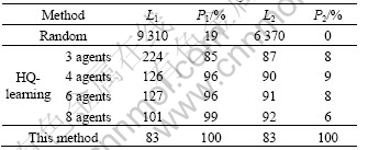
Table 1 lists the results of 100 simulations for “the key and the door” task with 3 different methods. The method proposed in this work can find optimal solution at each final trial. Therefore, considering the final test trial with the method proposed in this work, the average steps per trial (L₁) is 83, the goal hit percentages (P₁) is 100%, the average path lengths (L₂) is equal to the average step, and the percentage of optimal solution (P₂) reaches 100%. HQ-learning can solve the task with a limit of steps per trial, the method proposed in this work can solve the task with a limit of 100 steps per trial, and random search needs a step limit. These results show that the method proposed in this work is quicker and more stable than HQ-learning.

Table 1 Results of 100 simulations for “key and door” task

4 Conclusions

1) The proposed APF model is a novel method for solving reinforcement learning problems. The method converts reinforcement learning model to artificial potential field method, which is done by considering each state an attractive or a repulsive source whose influence strength is the temporal reward received by agent at the state. The local minimum problem for the APF model is solved by virtual water-flow technique. It is of great importance that at each trial the agent remembers the newest potential at the local minima, thus an optimal solution can be obtained in the following trials. The simulation of the key and door maze shows that this new method is simple and effective to give an optimal solution to the reinforcement learning problem.

2) The disadvantage of this method is that the agent has to know the exact states or observations of its neighbors, so that the neighbor potentials can be estimated more exactly. In the future work, the following problems should be considered: some theoretical works will be required to prove the convergence of algorithms and computational complex analysis of this method; the neighbor states or observations should be estimated exactly and efficiently; the performance of method needs to be tested in the environment of large-scaled unknown dynamic robots.

References

[1] KAELBLING L P, LITTMAN M L, MOORE A W. Reinforcement learning: A survey [J]. Journal of Artificial Intelligence Research, 1996, 4(1): 273-285.

[2] SUTTON R S, BARTO A. Reinforcement learning: An introduction [M]. Cambridge: MIT Press, 1998.

[3] BANERJEE B, STONE P. General game learning using knowledge transfer [C]// Proceedings of the 20th International Joint Conference on Artificial Intelligence. California: AAAI Press, 2007: 672-677.

[4] ASADI M, HUBER M. Effective control knowledge transfer through learning skill and representation hierarchies [C]// Proceedings of the 20th International Joint Conference on Artificial Intelligence. California: AAAI Press, 2007: 2054-2059.

[5] KONIDARIS G, BARTO A. Autonomous shaping: Knowledge transfer in reinforcement learning [C]// Proceedings of the 23rd International Conference on Machine Learning. Pittsburgh: ACM Press, 2006: 489-496.

[6] MEHTA N, NATARAJAN S, TADEPALLI P, FERN A. Transfer in variable-reward hierarchical reinforcement learning [C]// Workshop on Transfer Learning at Neural Information Processing Systems. Oregon: ACM Press, 2005: 20-23.

[7] WILSON A, FERN A, RAY S, TADEPALLI P. Multi-Task reinforcement learning: A hierarchical Bayesian approach [C]// Proceedings of the 24th International Conference on Machine Learning. Oregon: ACM Press, 2007: 923-930.

[8] GOEL S, HUBER M. Subgoal discovery for hierarchical reinforcement learning using learned policies [C]// Proceedings of the 16th International FLAIRS Conference. Florida: AAAI Press, 2003: 346-350.

[9] TAYOR M E, STONE P. Behavior transfer for value-function-based reinforcement learning [C]// The Fourth International Joint Conference on Autonomous Agents and Multiagent Systems. New York: ACM Press, 2005: 53-59.

[10] HENGST B. Discovering hierarchy in reinforcement learning with HexQ [C]// Proceedings of the 19th International Conference on Machine Learning. San Francisco: Morgan Kaufmann, 2002: 243-250.

[11] DIUK C, STREHL A L, LITTMAN M L. A hierarchical approach to efficient reinforcement learning in deterministic domains [C]// Proceedings of the 5th International Joint Conference on Autonomous Agents and Multiagent Systems. New York: ACM Press, 2006: 313-319.

[12] ZHOU W, COGGINS R. A biologically inspired hierarchical reinforcement learning system [J]. Cybernetics and Systems, 2005, 36(1): 1-44.

[13] BARTO A, MAHADEVAN S. Recent advances in hierarchical reinforcement learning [J]. Discrete Event Dynamic Systems: Theory and Applications, 2003, 13(1): 41-77.

[14] KEARNS M, KOLLER D. Efficient reinforcement learning in factored MDPs [C]// Proceedings of the 6th International Joint Conference on Artificial Intelligence. Stockholm: Morgan Kaufmann, 1999: 740-747.

[15] WEN Zhi-qiang, CAI Zi-xing. Global path planning approach based on ant colony optimization algorithm [J]. Journal of Central South University of Technology, 2006, 13(6): 707-712.

[16] ZHU Xiao-cai, DONG Guo-hua, CAI Zi-xing. Robust simultaneous tracking and stabilization of wheeled mobile robots not satisfying nonholonomic constraint [J]. Journal of Central South University of Technology, 2007, 14(4): 537-545.

[17] ZOU Xiao-bing, CAI Zi-xing, SUN Guo-rong. Non-smooth environment modeling and global path planning for mobile robots [J]. Journal of Central South University of Technology, 2003, 10(3): 248-254.

[18] ANDREWS J R, HOGAN N. Impedance control as a framework for implementing obstacle avoidance in a manipulator [C]// Proceedings of Control of Manufacturing Process and Robotic System. New York: ASME Press, 1983: 243-251.

[19] KHATIB O. Real-time obstacle avoidance for manipulators and mobile robots [J]. International Journal of Robotics Research, 1986, 5(1): 90-98.

[20] HUANG W H, FAJEN B R, FINK J R. Visual navigation and obstacle avoidance using a steering potential function [J]. Journal of Robotics and Autonomous Systems, 2006, 54(4): 288-299.

[21] PARK M G, LEE M C. Artificial potential field based path planning for mobile robots using a virtual obstacle concept [C]// Proceedings of IEEE/ASME International Conference on Advanced Intelligent Mechatronics. Victoria: IEEE Press, 2003: 735-740.

[22] LIU C Q, KRISHNAN H, YONG L S. Virtual obstacle concept for local-minimum-recovery in potential-field based navigation [C]// Proceedings of the IEEE International Conference on Robotics & Automation. San Francisco: IEEE Press, 2000: 983-988.

[23] BROCK O, KHATIB O. High-speed navigation using the global dynamic window approach [C]// Proceedings of the IEEE International Conference on Robotics and Automation. Detroit: IEEE Press, 1999: 341-346.

[24] KONOLIGE K. A gradient method for real time robot control [C]// Proceedings of the IEEE/RSJ International Conference on Intelligent Robots and Systems. Victoria: IEEE Press, 2000: 639-646.

[25] RIMON E, KODITSCHEK D. Exact robot navigation using artificial potential functions [J]. IEEE Transactions on Robotics and Automation, 1992, 8(5): 501-518.

[26] WIERING M, SCHMIDHUBER J. HQ-learning [J]. Adaptive Behavior, 1998, 6(2): 219-246.

Foundation item: Projects(30270496, 60075019, 60575012) supported by the National Natural Science Foundation of China

Received date: 2007-12-28; Accepted date: 2008-03-11

Corresponding author: CHEN Huan-wen, Professor; Tel: +86-731-2782298; E-mail: huanwen.chen@gmail.com

(Edited by CHEN Wei-ping)