高频尺度下基于符号时间序列的金属期货价格波动预测及实证
来源期刊:中国有色金属学报(英文版)2020年第6期
论文作者:吴丹 黄健柏 钟美瑞
文章页码:1707 - 1716
关键词:高频;铜;金属期货;符号时间序列;价格波动;预测
Key words:high-frequency; copper; metal futures; symbolic time series; price fluctuation; prediction
摘 要:构建高频尺度下的基于符号时间序列的金属期货价格波动预测模型,并选取上海铜期货交易所2014年7月到2018年9月的高频数据,采用符号时间序列方法将样本分为194个直方图时间序列,分别使用K-NN算法与指数平滑法预测下一个周期。结果显示,铜期货的收益预测得出的直方图走势比实际的直方图走势较为平缓,预测结果的整体情况较好,并且预测铜期货所得一周收益的整体波动与实际波动值在很大程度上一致。这表明用K-NN算法预测所得的结果比指数平滑法预测的结果更加精确。根据预测得到的铜期货一周的价格整体波动情况,中国铜期货市场的监管者及投资者可以及时调整其监管政策和投资策略以控制风险。
Abstract: The metal futures price fluctuation prediction model was constructed based on symbolic high-frequency time series using high-frequency data on the Shanghai Copper Futures Exchange from July 2014 to September 2018, and the sample was divided into 194 histogram time series employing symbolic time series. The next cycle was then predicted using the K-NN algorithm and exponential smoothing, respectively. The results show that the trend of the histogram of the copper futures earnings prediction is gentler than that of the actual histogram, the overall situation of the prediction results is better, and the overall fluctuation of the one-week earnings of the copper futures predicted and the actual volatility are largely the same. This shows that the results predicted by the K-NN algorithm are more accurate than those predicted by the exponential smoothing method. Based on the predicted one-week price fluctuations of copper futures, regulators and investors in China’s copper futures market can timely adjust their regulatory policies and investment strategies to control risks.
Trans. Nonferrous Met. Soc. China 30(2020) 1707-1716
Dan WU1,2, Jian-bai HUANG1,2, Mei-rui ZHONG1,2
1. School of Business, Central South University, Changsha 410083, China;
2. Institute of Metal Resources Strategy, Central South University, Changsha 410083, China
Received 11 February 2020; accepted 25 May 2020
Abstract: The metal futures price fluctuation prediction model was constructed based on symbolic high-frequency time series using high-frequency data on the Shanghai Copper Futures Exchange from July 2014 to September 2018, and the sample was divided into 194 histogram time series employing symbolic time series. The next cycle was then predicted using the K-NN algorithm and exponential smoothing, respectively. The results show that the trend of the histogram of the copper futures earnings prediction is gentler than that of the actual histogram, the overall situation of the prediction results is better, and the overall fluctuation of the one-week earnings of the copper futures predicted and the actual volatility are largely the same. This shows that the results predicted by the K-NN algorithm are more accurate than those predicted by the exponential smoothing method. Based on the predicted one-week price fluctuations of copper futures, regulators and investors in China’s copper futures market can timely adjust their regulatory policies and investment strategies to control risks.
Key words: high-frequency; copper; metal futures; symbolic time series; price fluctuation; prediction
1 Introduction
The price volatility, yield modeling and prediction of financial futures market trends constitute the main barriers to making accurate predictions of the capital market, as they provide a theoretical basis for financial pricing, multi-asset allocation, and financial risk management. The daily, weekly and monthly data of lower frequency were used to indirectly describe financial market price fluctuations and yield fluctuations by modeling the variance in earning conditions. In recent years, the acquisition of big data and high-frequency data have been possible with the development of financial technologies. The modeling, measurement and prediction of fluctuations in financial assets based on big data and high-frequency data have become a new focus of research. High-frequency data were mainly modeled based on realized volatility trends [1-4] as proposed by ANDERSEN and BOLLERSLEV [2] and nonparametric methods were mainly used to measure high-frequency fluctuations to avoid parameter estimation difficulties. After converting fluctuations into an observable time series based on realized wave theory, a high-frequency time series can be modeled using the conventional time series techniques: the first realized volatility methods developed include the autoregressive moving average model (ARMA) and the heterogeneous autoregressive model (HAR) [5,6]. GONG and LIN [7] studied structural breaks and volatility forecasting in the copper futures market. KANG and YOON [8] used the FIAPARCH model to test the long-term memory characteristics of high- frequency data on KOSPI 200 in Korea, and WANG [9] studied high-frequency data from the
Financial Times 100 Index and found the predictive ability of his HAR-RV model to be superior to that of other traditional conditional fluctuation models. ZHU et al [10-13] used the commodity spillover index model to empirically test price linkage changes in copper futures for major futures markets, analyzed the copper futures market and concluded the price fluctuations in China’s copper futures market. DAW et al [14] constructed a price prediction model with high-frequency copper futures data of Shanghai measured at intervals of 5 min. However, all of the future trading variables and volatility were predicted based on point predictions, so certain limitations in accurately and comprehensively revealing laws that govern high-frequency fluctuations in financial assets are shown. SHI et al [15] did empirical research to investigate the relationship between trading volume components and various realized volatility using 1 min high-frequency data of Shanghai copper and aluminum futures. WANG et al [16] constructed a structural vector autoregression (SVAR) model to investigate the direction and strength of the effects of influence factors on the international gold futures prices and the variance decomposition approach (VDA) was used to compare the contributions of these factors.
To make up for the shortcomings in overall fluctuations in financial asset prices and return rates, symbolic time series were widely used to analyze the overall distribution of financial asset prices and yield fluctuations and their volatility. Symbolic time series are new data analysis tools based on the theory of nonlinear dynamics developed from symbolic dynamics theory, chaotic time series analysis methods and information theory. The method is insensitive to noise, disturbances, etc. and dynamic characteristics of a system can be maintained such as correlation, periodicity, and complexity, which greatly improve the stability of financial data analysis. Symbolic time series have long been used in the fields of natural science and engineering [17-19]. In recent years, they have gradually been applied to researching on capital markets and economics. BRIDA and RISSO [20] classified US listed companies with asset returns and transaction volumes to determine stock market structures using symbolic time series and multi- dimensional minimum span trees. BRIDA et al [21] studied the synergistic motion relationship between time series of different exchange rates and the contagiousness of currency crises using symbolic time series and hierarchical trees. XU and HUANG [22] introduced symbolic time series to empirically analyze the earning series of six stock indices, determined the main change patterns of each index’s earnings, and predicted earnings based on major trends. ARROYO and MATE [23] proposed an exponential smoothing method based on a histogram algorithm to predict the histogram series. ARROYO and MATE [24] used the K-NN algorithm to predict the histogram series, applied this method to studying financial data and found the prediction results of K-NN algorithm to be more accurate than those predicted using other models. XU [25] combined a symbolic time series analysis with the K-NN algorithm to propose a prediction method for the overall distribution of high- frequency financial fluctuations based on a symbolic time series histogram. XU and SHEN [26] constructed a financial anomaly fluctuation model based on the symbolic time series method and empirically analyzed the effectiveness relationships of user markets. LIU and GONG [27] analyzed time-varying volatility spillovers between the crude oil markets using a new method. LI and LIANG [28] constructed a model to measure time series similarities in numerical symbols and morphological features.
In the context of the new normal of China’s economy, price fluctuations in the metal futures market are becoming more frequent and intense. Therefore, it is particularly important to predict the overall volatility of a cycle of metal futures prices. However, little has been done on this issue in the existing research. Therefore, an in-depth study on the overall one-week volatility in the metal futures price was conducted. Taking Shanghai’s copper futures market as an example, five-time-sharing transactions data on copper futures from July 2014 to September 2018 was used as a sample, the fluctuation series of copper futures were symbolized and the distribution of the symbolic series was visualized with a symbolic series histogram. Then the overall distribution of high- frequency copper futures price fluctuations was predicted by the K-NN algorithm and exponential smoothing respectively and in turn the feasibility and effectiveness of the new method were verified. Compared with previous prediction models, the model proposed in this study has higher prediction accuracy.
2 Framework of high-frequency symbolic time series of price fluctuation predictions
2.1 Theoretical modeling for symbolic time series of price fluctuations
The conversion of raw data for price fluctuation predictions is a process of symbolization that uses symbolic time series to conduct predictive analyses. Raw data used for price fluctuation predictions have basic global attributes: certainty, complexity, periodicity, and so on. To compromise the complexity and periodicity of the raw data, the symbolization of time series should be divided into the following steps. First, segment the phase space of the original data finitely. Then, convert it into a series of symbols including only a limited number of values by assigning a simple symbol to each series segment. The focus of price fluctuation symbolization is to determine the segmentation position by equal probability segmentation and to then determine the number of price fluctuation symbols.
Given the price fluctuation time series t={t1, t2, …, tN} and segmentation position p={p1, p2, …, pn+1}, the symbolic series of price fluctuations is recorded as s={s1, s2, …, sN}, and then the price fluctuation symbolization rule is sj={j-1|pi≤tj
i+1, i=1, 2, …, n, j=1, 2, …, N}. To calculate statistics for the symbolic series of price fluctuations more easily, we encode them and determine an appropriate word length, take a continuous symbol from the symbolic time series of price fluctuations to form a word, and employ modified Shannon entropy. For a series with n symbols and a word length of L, the modified Shannon entropy formula is written as
 (1)
(1)
where Nobs is the number of different words appearing in the symbolic series of price fluctuations. Rather, the number of words whose probability of occurrence is nonzero, Nobs≤nL, i is the number of the word, and Pi,L is the probability of the ith word with a word length of L appearing. (1) Let the word length be L, which is a variable. Draw L consecutive symbolic data in order from the symbolic series of price fluctuations {sj} to compose a word and to form a new sequence, which is recorded as {sksk+1…sk+L-1, k=1, 2, …, N+1+L}. (2) Encode {sksk+1…sk+L-1, k=1, 2, …, N+1+L}, and then we have {Ck|Ck=sk+Ln0+ sk+L-2n1+…+sknL-1, k=1, 2, …, N+1-L }, which is the coding sequence formed by the decimal sequence code. (3) Calculate the probability values of different words and the number of words with nonzero probability when the number of symbols is n, and the word length is L according to the decimal coding sequence {Ck}. Equation (1) is used to calculate the modified Shannon entropy value corresponding to different word lengths L, and then the word length corresponding to the lowest entropy value is what should be selected.
After selecting an appropriate word length, here we determine the probability of each word occurring to facilitate the prediction of the symbolic time series of the next cycle of price fluctuations. As a result, the price series of metal futures are symbolized and the probability distribution histograms for each different wave pattern are obtained.
2.2 K-NN prediction algorithm for symbolic time series of price fluctuations
2.2.1 Principles of K-NN prediction algorithm for symbolic time series of price fluctuations
This study uses K-NN (K-Nearest Neighbors) as the prediction tool of the price fluctuation histogram time series. When most of the k most similar samples in the feature space are of a certain category, the sample also belongs to this category. In the K-NN algorithm, the selected neighbors are objects that have been correctly classified. Since the selection of dimensions often affects the accuracy of results when using the K-NN algorithm for predictions, the G-P method is used to obtain the best dimension by phase space reconstruction. (1) Construct a histogram time series of price fluctuations  where t=1, 2, …, n, according to which construct a d-dimensional histogram vector time series
  where =(,
  , …,
, …,  ), t=d, …, n; (2) Calculate the distance between the histogram vector
  =(
=( ,
,  , …,
, …,  ), which is closest to
  and all other d-dimensional histogram vectors. The formula isthen:
  (3) Calculate the distance between
  and each (where t=T-1, T-2, …, d) according to step 2, and select k vectors which are the closest to and which are marked as
  ,
,  , …,
, …,  . (4) According to the k nearest histogram vectors of price fluctuations obtained in step 3, take the weighted average of
  histogram variables of the k vectors, and the final predicted value
  is then

 (2)
(2)
where ξ is 10-5, mainly to prevent the distance between the two series histogram sequences of price fluctuations being valued at zero.  is the distance,
  is a variable of the next histogram of price fluctuations of the continuous subsequence
  , and ωp is the weight of the neighbor p, which satisfies ωp≥0 and
  . Assuming that all price fluctuation neighbors have the same weight, ωp=1/k.
2.2.2 Distance of symbolic histogram sequence of price fluctuations
In applying the K-NN algorithm, the selection of a formula measuring the distance between symbolic histogram sequences of price fluctuations is particularly important. We use the Euclidean distance formula for two symbol sequence histograms X and Y written as
 (3)
(3)
The probability of occurrence of the word i in histograms X and Y, K is the total number of all possible words in X and Y, and L is the word length. OXY(L) measures the distance between two histograms by measuring the difference between the probabilities of all words that could be included in the two histograms of price fluctuation symbol sequences. The shorter the distance is, the more similar the dynamic characteristics of the two sequences are. Therefore, OXY(L) can be used to measure the similarities between two symbol sequences of price fluctuations.
The symbolic histogram sequence of price fluctuations is composed of symbolic sequence histograms observed at different time. For two symbolic histogram series of the same time length d: t=1, 2, …, d},
  t=1, 2, …, d}, where
  …,
…, and
and  =
=
 …,
…,  . The Euclidean norm is defined as
 (4)
(4)
2.2.3 Selection of the best dimension m of price fluctuations
Dimension m is an important variable in the application of the K-NN algorithm. The key point of the selection is to delay embedding for efficient spatiotemporal conversion. Let the time series of price fluctuations observed be x1, x2, …, xn and appropriately select a time delay value τ. Construct an m-dimensional phase space of price fluctuations, the vector of which is Xi=(Xi, Xi+τ, …, Xi+(m-1)τ), i=1, 2, …, N, N=n-(m-1)τ. n is the number of points in the original time series of price fluctuations. The method described above is used to construct N m-dimensional vectors, and m is then called the embedded dimension. When m≥2d+1 (d is the dimension of the attractor in the original space), the trajectories described by N vectors in the m-dimensional phase space can reproduce geometric features of the original attractors. The single variable sequence of price fluctuations can reconstruct overall properties of the system due to interactions that occur between various variables in a nonlinear system. A change in a variable must be affected by other variables (of course, the degree of strength will vary). For long-term observations, the univariate sequence must contain information of other variables involved in the dynamic system. When the data are sufficient and without noise interference and when the chosen embedding dimension m and delay time τ are appropriate, it should be possible to grasp the overall situation. By examining how the number of points in the radius-k sphere embedded in space decreases to zero with the radius, the value of the fractal dimension can be estimated from the experimental time series. First, define the correlation function C(r) as
 (5)
(5)
where θ(x) is a step function defined as
 (6)
(6)
where |Xi-Xj| represents the distance between state vectors Xi and Yj in Euclidean space, N denotes the number of points in the phase space, and C(r) represents the ratio of the number of pairs of points in the phase space positioned less than r from all possible pairs of points, denoting the probability of the distance between two points on the attractor in the phase space being less than r and characterizing the degree of point convergence. When a constant D2 causes the correlation function C(r) to obey the following scale law, it essentially depicts similarities that may exist in phase space. When  , then D2 is called the correlation dimension, and the reconstructed attractor has the fractal feature. The correlation dimension D2 is defined as
 (7)
(7)
Therefore, to obtain a constant correlation dimension D2 in a system, we can draw a double logarithmic curve of ln C(r) relative to ln r, from which we find the slope of a relatively long and nearly straight segment (forming the scale-free region). When the slope of the curve gradually converges to a saturated value as the embedding dimension m gradually increases, then the limit is called the true correlation dimension D2. For a purely stochastic process, the slope will increase as the embedding dimension m increases, and it will not converge to a saturated value. That is, there is no fractal structure, and the system is not a chaotic system.
2.3 Exponential smoothing method for price fluctuation prediction
The purpose of exponential smoothing for price fluctuation prediction is to smooth out the time series of price fluctuations to eliminate irregular and random disturbances using a weighted average method assuming that the impact of recent data in time series of price fluctuations on future values is stronger than that of earlier data. Therefore, when weighting data of a time series of price fluctuations, the more recent the data area, the larger the weight and vice versa. This smooths the data and reflects the influence on the value of the predicted point in a time series of price fluctuations. According to smoothing requirements, there may be one, two or even three rounds of exponential smoothing. Let the symbolic time series of price fluctuations be x1, x2, x3, …, xN. As a result, the recurrence formula for an exponential smoothing sequence is
 0<α<1, 1≤t≤N (8)

where  represents the value of exponential smoothing at point t, and α is the smoothing coefficient. The initial value of the recurrence formula
  is the first item of the common time series (applicable to a large collection of historical data points such as 50 or more). If the size of the historical dataset is small, including 15 or 20 data points or less, the average of historical data for the first few weeks can be used as the initial value . These approaches are somewhat empirical and subjective.
We next discuss the smoothing factor α and expand the recursive formula to


 (9)
(9)
As 0≤α≤1, coefficient α(1-α)i of xi decreases as i increases. Note that the sum of these coefficients is 1, where 

 . Thus, in the recursive formula is a weighted average of the sample values x1, x2, x3, …, xt. When we use the recursive formula to predict price fluctuations, is used as the predicted value of point t+1. The above discussion shows that weight of xt of time point t most closely reflecting predicted time point t+1 is α, which is the largest, and for xt-1, the weight is α(1-α), x1 is the smallest. We find that the formula produces a weighted average for the original time series when recent data are considered to have strong impact on the future while long-term data are considered to have a limited effect. When the smoothing coefficient α=0,
  the smoothing value of each time point is equal to after determining
  . At this point, the observed value xi of each time point i has no effect. When the smoothing coefficient α=1,
  , the smoothed sequence is the original time series, and no processing or smoothing is performed on the original time series. For the smoothing coefficient α, the coefficients of xi and xj (i≠j) cannot be equal except under the above two extreme conditions.
In summary, when 0<α<1 and is close to 1, the calculated smoothness value of an exponent of price fluctuations is less uniform with the original historical data, and of the smoothed sequence can reflect the actual change to the original time series relatively quickly. Therefore, for a time series of price fluctuations with considerable changes or strong trends, it is suitable to select data with smoothing coefficients of close to 1 such as α=0.95, 0.90. When 0<α<1 and the value is close to 0, the calculated smoothing value will be more uniform with the original historical data, and the smoothed sequence will not be sensitive to the original time series. Therefore, for time series showing few or no changes in price fluctuations, we should use a smoothing coefficient close to 0 to render the weights of the data relatively similar during the smoothing process.
2.4 Measuring accuracy of symbolization predictions of price fluctuations
When predicting a high-frequency histogram sequence  of metal futures price fluctuations whose result is denoted as
  , then the prediction error is
  but
but  cannot discern the quantitative difference between
  and
and  or how larger the error value is. At this point, it is necessary to introduce the MDE (mean distance error) to quantify the error, which is usually written as
 (10)
(10)
where  can be different formulas of distance and T is the number of cycles predicted. The selection of the error formula often has a great influence on the accuracy of calculation results. We compare two relatively mature error formulas.
(1) Mean absolute error
 (11)
(11)
(2) Mean square error
 (12)
(12)
3 Empirical analysis of symbolic time series of price fluctuations predictions
3.1 Preprocessing of price fluctuation data
We collect five-time-sharing transaction data for copper futures from July 2014 to September 2018. Since the delivery month is close to the spot delivery date, the future price is greatly affected by the spot price. In our empirical analysis, we use the daily settlement price of futures contracts created three months away from the delivery month to form a continuous price sequence. The futures contracts have the largest trading volumes and numbers of market participants and exhibit the most active levels of trading, which is enough to reflect the group will of market participants, and the artificial manipulation of the price can be prevented by the settlement price. To predict the one-week distribution of copper futures price fluctuations, the data are grouped from Monday-Friday where each week is grouped and data on less than 1000 weeks are excluded. We obtain 194 sets of transaction data, each of which forms a weekly sequence, and there are 284 data points in weekly sequence. The income at t of the ith week is defined as Rti=lg Pt,i- lg Pt-1,i where i=1, 2, …, 194, and price fluctuations are defined as the square of the income or as  .
.
3.2 Obtaining symbol histogram time series of price fluctuation predictions
First, symbolize the copper futures price fluctuation sequence of each cycle {υti, t=1, 2, …, 284}(i=1, 2, …, 194) via equal probability division. We adopt 3 symbols and the following division rules:
 (13)
(13)
where υ1/3i and υ2/3i respectively represent the one-third and two-thirds quantiles of {υti}. Thus, 0, 1 and 2 correspond to low, moderate and high intervals, respectively, and the copper futures price fluctuation sequence of each cycle is written as: {Sti, t=1, 2, …, 284}(i=1, 2, …, 194). Then, we use the minimum entropy rule of modified Shannon entropy to determine the appropriate word length as in Eq. (1) to apply a word length and to render the improved Shannon entropy value the lowest under the determined number of symbols, where L is an integer among [2,6]. As our goal is to improve the Shannon entropy of the weekly symbolic sequence of copper futures price fluctuations, when comparing the entropy values of different word lengths, we can compare mean values of the entropy of different word lengths as
 L∈{2, …, 6} (14)
We find that when the word length L increases, H(L) decreases continuously, but the rate of decrease slows. From the limit on the number of samples of copper futures price series for each cycle, the word length should be equal to the number obtained. We calculate the frequency corresponding to different words when L is equal to the number obtained from the symbolic sequence of copper futures price fluctuations of each cycle, {Sti, t=1, 2, …, 283}(i=1, 2, …, 194). In turn, we obtain a symbolic sequence histogram of copper futures price fluctuations for each cycle, all of which form a symbolic histogram time series written as {hxt, t=1, 2, …, 194}. The results calculated with the above method are shown in Table 1.
Table 1 Average entropy of symbolic time series of copper futures returns

After symbolizing the weekly copper futures price return, we obtain a symbolized series of weekly copper futures price returns from 194 weeks of data. According to the description given above, word lengths vary from Refs. [2,6], and we then calculate the weekly Shannon entropy of different word lengths L and average the entropy values of all weeks to obtain an average Shannon entropy value. Table 1 shows that the entropy value decreases from 2 and then reaches a minimum value of 0.9667 at L=4, after which the S entropy value begins to increase again. Thus, L=4 is the best word length.
3.3 Selecting the best dimension from G-P algorithm
We use the G-P algorithm to determine the embedding dimension, and the best dimension is obtained under the assumed condition of τ=1. Figure 1 presents a double logarithmic curve of ln C(r) and ln r of the symbolic sequence of copper futures returns, and Fig. 2 presents a graph of the correlation dimension. It can be observed from Fig. 2 that the slope of the double logarithmic curves of ln C(r) and ln r tends to a saturated value when Dm=3.2, at which the geometric attractor of the system reaches a state of the maximum saturation. The best embedding dimension is then calculated based on the best embedding dimension as m≥2Dm+1.

Fig. 1 Double logarithmic curve of ln C(r) and ln r of copper futures symbol sequence (C(r) is the probability that the distance between two points on the attractor in phase space is less than r)

Fig. 2 Correlation dimension of return symbols time series (Dm is the limit of the slope of the logarithmic curve as r approaches 0)
It can be observed from Fig. 1 and Fig. 2 that when m is low, the slope of the straight-line segment of the double logarithmic curve (i.e., the correlation dimension) increases as m increases. When m=9-20, the slope of the curve nearly plateaus at close to 3.26, and the correlation dimension is saturated for the first time. Therefore, according to the saturation correlation dimension approach, the minimum embedding dimension corresponding to the correlation dimension of 3.26 is int(2D+1)=8.
3.4 Prediction and accuracy of copper futures price fluctuation measurements
After processing copper futures price data according to the method shown above, we obtained a 194-week symbolic time series xt(t=1, 2, …, 194). Then the symbolic time series for 194 weeks are divided into two intervals:  ={x1, x2, …, x184} for prediction and
  ={x185, x186, …, x194} for testing. The mean absolute error (MAE) of Eq. (12) and the mean square error (MSE) of Eq. (13) are taken as the standard for error calculations in predicting copper futures price fluctuations. While making predictions, similarities observed between copper futures price fluctuation histograms are measured from the Euclidean distance. To examine the different prediction results of methods, the K-NN and exponential smoothing algorithms are used to process the experimental data on copper futures price fluctuations, and the 10-week prediction results for copper futures price fluctuations are written as
  ={z1, z2, …, z10} and
  ={y1, y2, …, y10}
(1) K-NN algorithm predictions
A comparison of predictions using the K-NN algorithm based on high-frequency data on copper futures price fluctuations and actual detection values is shown in Figs. 3 and 4, where each histogram corresponds to the one-week symbolic time sequence of the copper futures return (returns vary within high, medium and low ranges). Figure 3 reflects the actual value and Fig. 4 reflects the predicted value.
Figure 4 shows that histogram trends of predicted copper futures returns are more gradual than those derived from actual observations, but the general trends are basically the same. This indicates that the prediction results are good overall. However, the probability distribution of fluctuations represented by each word in the copper futures return prediction histogram is more gradual than the real distribution (Fig. 4). This gradual nature may occur because the predicted histogram reflects a weighted average of k histograms.
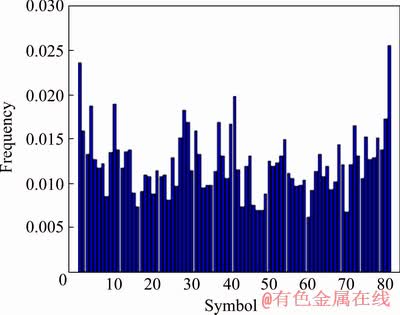
Fig. 3 Histogram of actual observations

Fig. 4 Histogram of K-NN algorithm predictions
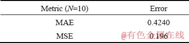
According to Table 2, no matter which metric is used, the MSE is always an order of magnitude smaller than the MAE. Thus, the prediction error of the copper futures return is within an acceptable range, showing that the K-NN prediction algorithm presented in this paper is suitable for the return data on copper futures and for analyzing return fluctuations of basic metal futures.
(2) Exponential smoothing predictions
In this section, we use the two interval datasets of the symbolic sequence of the copper futures return processed above ={x1, x2, …, x184}, and we use  ={x185, x186, …, x194} to predict the 10-week symbolic sequence of copper futures returns. Figure 6 shows a histogram of weekly predictions. α is a very important parameter when using the exponential smoothing method, and its most suitable value is α=0.0355 as obtained with general statistical tools, at which the error value is the smallest. It can be observed from Fig. 6 that the main trends are consistent but are not as optimized as the results of K-NN prediction algorithm, indicating that the method still presents shortcomings in generating symbolic time series of copper futures returns.
Table 2 Prediction errors of K-NN algorithm

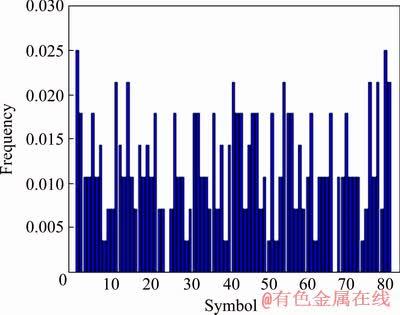
Fig. 5 Histogram of week actual observations

Fig. 6 Histogram of exponential smoothing predictions
Table 3 presents the prediction error of the exponential smoothing method, which is significantly larger than that of the K-NN algorithm shown in Table 2. Therefore, the exponential smoothing prediction algorithm is not as effective as the K-NN algorithm, and the latter is more suited to addressing symbolic time sequences of copper futures returns.
Table 3 Prediction error of exponential smoothing algorithm
4 Conclusions
(1) The overall error value of predictions of copper futures price fluctuations falls within an acceptable range, and thus the symbolic time series can effectively fit high-frequency fluctuations in copper futures prices.
(2) The trend of the histogram derived from the copper futures earnings prediction is gentler than the actual histogram, the overall situation of the prediction results is better, and the model has higher accuracy.
(3) The results predicted by the K-NN algorithm are more accurate than those predicted by the exponential smoothing method. The results show that the overall error value of predictions of copper futures price fluctuations falls within an acceptable range, and thus the symbolic time series can effectively fit high-frequency fluctuations in copper futures prices.
References
[1] ADMATI A R, PFEIDERER P. A theory of intraday patterns: Volume and price variability [J]. The review of financial studies, 1988, 1(1): 3-40.
[2] ANDERSEN T G, BOLLERSLEV T. Answering the skeptics: Yes, standard volatility models do provide accurate forecasts [J]. International Economic Review, 1998(39): 885-905.
[3] ANDERSEN T G, BOLLERSLEY T. DM-dollar volatility: intraday activity patterns, macroeconomic announcements, and longer run dependencies [J]. Journal of Finance, 1998, 1(53): 219-265.
[4] TANG Yong, LIN Xin. Volatility modeling in consideration of the Co-jumps: Based on the perspective of high-frequency data [J]. Chinese Journal of Management Science, 2015(8): 46-53. (in Chinese)
[5] ANDERSEN T G, BOLLERSLEV T, DIEBOLD F X, ANDERSEN T G, BDLLERSLEV T, DIEBOLD F X, LABYS P. Modeling and forecasting realized volatility [J]. Econometrical, 2003, 71(2): 579-625.
[6] CORSI F. A simple approximate long-memory model of realized volatility [J]. Journal of Financial Econometrics, 2009, 7(2): 174-196.
[7] GONG Xu, LIN Bo-qiang. Structural breaks and volatility forecasting in the copper futures market [J]. Journal of Futures Markets, 2018, 38(3): 290-339.
[8] KANG S H, YOON S M. Long memory features in the high frequency data of the Korean stock market [J]. Physica A: Statistical Mechanics and its Applications, 2008, 387(21): 5189-5196.
[9] WANG Peng. Modeling and forecasting of realized volatility based on high-frequency 44 data: evidence from FTSE-100 index [R]. Vaasa: Hanken School of Economics, 2009.
[10] ZHU Xue-hong, CHEN Jin-yu, SHAO Liu-guo. Research on the international pricing ability of China's metal futures market from the perspective of information spillover [J]. Chinese Management Science, 2016, 24(9): 28-35. (in Chinese)
[11] ZHU Xue-hong, CHEN Qiang, CHEN Jin-yu. Research on dynamic correlation of copper-aluminum futures based on high frequency volatility [J]. Commercial Research, 2017, 2: 50-57. (in Chinese)
[12] ZHU Xue-hong, ZHANG Hong-wei, ZHONG Mei-rui, LIU Hai-bo. Research on the relationship between volume and price of Chinese nonferrous metal futures market based on high frequency data [J]. Chinese Management Science, 2018, 26(6): 8-16. (in Chinese)
[13] ZHU Xue-hong, ZOU Jia-wen, HAN Fei-yan, CHEN Jin-yu. Modeling and prediction of high frequency volatility in China's copper futures market with external impacts [J]. Chinese Management Science, 2018, 26(9): 52-61. (in Chinese)
[14] DAW C S, FINNEY C E A, TRACY E R. A review of symbolic analysis of experimental data [J]. Review of Scientific instruments, 2003, 74(2): 915-930.
[15] SHI Bai-sheng, ZHU Xue-hong, ZHANG Hong-wei, ZENG Yi. Volatility-volume relationship of Chinese copper and aluminum futures market [J]. Transactions of Nonferrous Metals Society of China, 2018, 28(12): 2607-2618.
[16] WANG Hao, SHENG Hu, ZHANG Hong-wei. Influence factors of international gold futures price volatility [J]. Transactions of Nonferrous Metals Society of China, 2019, 29 (11): 2447-2454.
[17] GONG Xu, LIN Bo-qiang. The incremental information content of investor fear gauge for volatility forecasting in the crude oil futures market [J]. Energy Economics, 2018, 74: 370-386.
[18] BRIDA J G, PUNZO L F. Symbolic time series analysis and dynamic regimes [J]. Structural Change and Economic Dynamics, 2003, 14(2): 159-183.
[19] GONG Xu, LIN Bo-qiang. Forecasting the good and bad uncertainties of crude oil prices using a HAR framework [J]. Energy Economics, 2017, 67: 315-327.
[20] BRIDA J G, RISSO W A. Multidimensional minimal spanning tree: The Dow Jones case [J]. Physica A: Statistical Mechanics and its Applications, 2008, 387(21): 5205-5210.
[21] BRIDA J G, GOMEZ D M, RISSO W A. Symbolic hierarchical analysis in currency markets: An application to contagion in currency crises [J]. Expert Systems with applications, 2009, 36(4): 7721-7728.
[22] XU Mei, HUANG Chao. Analysis and prediction of financial returns based on symbolic time series method [J]. Chinese Management Science, 2011, 9(5): 1-9. (in Chinese)
[23] ARROYO J, MATE C. Exponential smoothing methods for histogram time series based on histogram arithmetic [R]. Madrid: Universidad Complutense de Madrid, 2008.
[24] ARROYO J, MATE C. Forecasting histogram time series with k-nearest neighbors methods [J]. International Journal of Forecasting, 2009, 25(1): 192-207.
[25] XU Mei. High-frequency financial fluctuation prediction based on symbol time series histogram [J]. Journal of Systems Management, 2014, 23(3): 332-338. (in Chinese)
[26] XU Mei, SHEN Lai-feng. Analysis of the relationship between financial anomaly fluctuation and market effectiveness based on symbolic time series method [J]. Mathematical Statistics and Management, 2015, 34(2): 357-366. (in Chinese)
[27] LIU Tang-yong, GONG Xu. Analyzing time-varying volatility spillovers between the crude oil markets using a new method [J]. Energy Economics, 2020, 87: 104711.
[28] LI Hai-lin, LIANG Ye. Measurement method of time series similarity based on numerical symbols and morphological features [J]. Control and Decision, 2017, 32(3): 451-458. (in Chinese).
吴 丹1,2,黄健柏1,2,钟美瑞1,2
1. 中南大学 商学院,长沙 410083;
2. 中南大学 金属资源战略研究院,长沙 410083
摘 要:构建高频尺度下的基于符号时间序列的金属期货价格波动预测模型,并选取上海铜期货交易所2014年7月到2018年9月的高频数据,采用符号时间序列方法将样本分为194个直方图时间序列,分别使用K-NN算法与指数平滑法预测下一个周期。结果显示,铜期货的收益预测得出的直方图走势比实际的直方图走势较为平缓,预测结果的整体情况较好,并且预测铜期货所得一周收益的整体波动与实际波动值在很大程度上一致。这表明用K-NN算法预测所得的结果比指数平滑法预测的结果更加精确。根据预测得到的铜期货一周的价格整体波动情况,中国铜期货市场的监管者及投资者可以及时调整其监管政策和投资策略以控制风险。
关键词:高频;铜;金属期货;符号时间序列;价格波动;预测
(Edited by Xiang-qun LI)
Foundation item: Projects (71633006, 7184207, 7184210) supported by the National Natural Science Foundation of China; Project (2019CX016) supported by the Annual Innovation-driven Project in Central South University, China
Corresponding author: Mei-rui ZHONG; Tel: +86-15874096280; E-mail: zmr726@163.com
DOI: 10.1016/S1003-6326(20)65332-8

