New algorithm for solving 3D incompressible viscous equations based on projection method

NIU Xiao-feng¹, LIANG Wei¹, ZHAO Yu-hong², HOU Hua², MU Yan-qing², HUANG Zhi-wei², YANG Wei-ming²

1. College of Materials Science and Engineering, Taiyuan University of Technology, Taiyuan 030024, China;

2. College of Materials Science and Engineering, North University of China, Taiyuan 030051, China

Received 16 September 2010; accepted 16 December 2010

Abstract: A new algorithm based on the projection method with the implicit finite difference technique was established to calculate the velocity fields and pressure. The calculation region can be divided into different regions according to Reynolds number. In the far-wall region, the thermal melt flow was calculated as Newtonian flow. In the near-wall region, the thermal melt flow was calculated as non-Newtonian flow. It was proved that the new algorithm based on the projection method with the implicit technique was correct through nonparametric statistics method and experiment. The simulation results show that the new algorithm based on the projection method with the implicit technique calculates more quickly than the solution algorithm-volume of fluid method using the explicit difference method.

Key words: implicit finite difference method; 3D incompressible viscous equations; projection method; nonparametric statistics

1 Introduction

Filling simulation is a very important and helpful tool for engineers to design casting process. Computational fluid dynamics (CFD) techniques, namely marker and cell (MAC) and solution algorithm-volume of fluid (SOLA-VOF) are found to be suitable to analyze the fluid flow problems. The SOLA-VOF method has advantage that the surface tension and wall adhesion can be evaluated from the orientation of free surface.

In the SOLA-VOF method, an explicit difference method is often used to calculate the 3D incompressible viscous equations in filling simulation. When δx, δy and δz are determined, the value of δt is limited by the numerical stability condition [1-3] (δx, δy and δz are the space steps, and δt is the time step). If the value of δt exceeds the stability condition, the mathematical operation becomes unstable. In many cases, because the time step is limited, the computational efficiency is low.

In this work, a new algorithm based on the projection method with the implicit finite difference technique was established to simulate the filling process.

The calculation region can be divided into different regions according to Reynolds number [4]. According to different regions, different forms of governing equations were used to calculate the velocity fields and the pressure for the first time. The simulation results show that this new algorithm calculates more quickly than the SOLA-VOF method using the explicit difference method.

2 Governing equations

The governing equations for 3D incompressible viscous flow contain mass conservation equation and momentum equations. The three-dimensional Cartesian coordinate is used [5-6].

The mass conservation equation is expressed as:

                             (1)

The momentum equation is expressed as:

 (2)

where t is time; is the velocity fields; p is pressure; S is the non-Newtonian part of the extra stress tensor; is the gravitational field; non-dimensional parametersand  are the Reynolds and Froude numbers; u₀ and L denote typical velocity and length;

ρ is density; μ is dynamic viscosity. In the far-wall region, the thermal melt flow has characteristics of Newtonian flow, so that the filling process can be calculated as Newtonian flow. In the near-wall region, the thermal melt flow has characteristics of non-Newtonian flow, so that the filling process can be calculated as non-Newtonian flow. For Newtonian flow, S=0,     this can be achieved by setting and. For non-Newtonian flow, S≠0, this can be achieved by setting α=λ₂/λ₁ and (λ₁ and λ₂ are relaxation and retardation time constants, respectively). In order to solve Eqs. (1) and (2), the staggered mesh is established.

3 Implicit finite difference method for thermal melt flow in far-wall region

In the far-wall region, the filling process is calculated as Newtonian flow. According to Eqs. (1) and (2), the general mathematical equations that 3D model of Newtonian incompressible viscous flow can be written as (,):

         (3)

                                    (4)

Based on the projection method, the implicit technique is used to solve Eqs. (3) and (4).

Eqs. (3) and (4) can be expressed for time step n+1 as:

            (5)

                                (6)

The velocity fields and pressure can be calculated by the following steps.

First, the basic idea behind this approach is to use Eq. (5) to solve the intermediate velocity field u.

               (7)

The momentum equation Eq. (7) can be approximated, the time term and viscous term can be gotten from Crank-Nicolson method, the pressure term is calculated by using forward differences, and the convective terms are calculated by the upwind scheme.

The momentum equations can be approximated by using the following finite difference equation in the X direction.

              (8)

where  equals +1 if  and -1 if ;. Other parameters are treated similarly. With obvious notation, similar expressions for the momentum equations can be readily obtained in Y and Z directions.

Second, this velocity fields are written as the following form by using Helmholtz-Hodge theory [5-15]:

                           (9)

Eq. (9) is written as component form:

                        (10)

Third, the pressure is computed. To obtain an equation for the pressure,  is introduced from Eq. (9) into Eq. (7) and then it is subtracted from Eq. (5) to obtain

                (11)

where. When  is calculated for each full cell, the pressure is gotten from the following finite difference equation:

             (12)

The intermediate velocity fields  can be calculated from Eq. (7), and the final velocity fields and the final pressure can be gotten from Eqs. (10) and (12).

4 Implicit finite difference method for thermal melt flow in near-wall region

In the near-wall region, the filling process can be calculated as non-Newtonian flow. The general mathematical equations can be written as (, ) [11-15]:

  (13)

                                   (14)

The implicit technique is used to solve Eqs. (13) and (14). Eqs. (13) and (14) can be written as

                (15)

                                (16)

The velocity fields and the pressure can be calculated by the following sequence of steps.

First, the basic idea behind this approach is to use Eq. (15) to solve the intermediate velocity field .

                 (17)

Second, Helmholtz-Hodge theory is used, and the velocity fields can be written as:

                          (18)

Third, the pressure is computed as:

             (19)

where; the stress tensor S can be solved from the Oldroyd-B constitutive equation as:

  (20)

where is the Weissenberg number.

5 Results and discussion

Gravity casting is adopted and the geometric

modeling is shown in Fig. 1. The pouring speed is    0.4 m/s and the pouring temperature is 720 °C. The physical parameters of the casting and mold are listed in Table 1. The simulation results of the new algorithm based on the projection method with the implicit finite difference technique are compared with the simulation results of the SOLA-VOF method using the explicit difference method. The explicit SOLA-VOF method is applied to some commercial simulation software and the validity of the explicit SOLA-VOF method is proved. Figure 2 illustrates both the experiment results and the simulation results of the new algorithm [16-17]. It is clear that the simulation results agree very well with the experiment results.

Fig. 1 Schematic dimensions of gravity casting model (Unit: mm)

The mesh size is 2.0 mm×2.0 mm×2.0 mm, and the total number of meshes is 40671. The process of comparison can be described as follows:

1) The simulation results of the same aluminum casting are calculated by the new algorithm and the SOLA-VOF method using the explicit difference method (identical parameter value).

The simulation results of the velocity field () and the pressure (p) are compared between the new algorithm and the SOLA-VOF method using the explicit difference method at simulated time of 1.0, 1.5, 2.0, 2.5 and 3.0 s, respectively.

2) Take the case of the velocity in X direction (at simulated time of 1.0 s).

The sample size is all the meshes. The method of the Wilcoxon signed rank test is used to compare the velocity between the new algorithm and the SOLA-VOF method using the explicit difference method in X direction.

The calculation results are listed in Table 2, where the last two rows are the ranks. The absolute rank row has no signs, and the signed rank row gives the ranks along with their signs [18].

Set the null and alternative hypotheses as: H0 is the simulation results are unanimous between the new algorithm and the explicit SOLA-VOF method. H1 is the simulation results are not unanimous between the new algorithm and the explicit SOLA-VOF method.

The test statistic is given by Refs. [18-22]:

   (21)

where .

There is no enough evidence to reject H0.

The simulation results () are analyzed in the same way (at simulated time of 1.0 s).

Other analyses are similar at simulated time of 1.5, 2.0, 2.5 and 3.0 s, respectively.

Analysis shows that the simulation results are unanimous between two methods. It is proved that the new algorithm is correct.

Table 1 Physical parameters of casting and mold

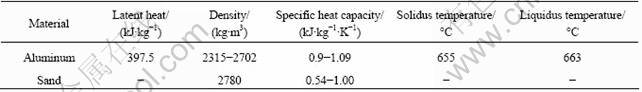
Table 2 Calculation results of new algorithm and explicit SOLA-VOF method

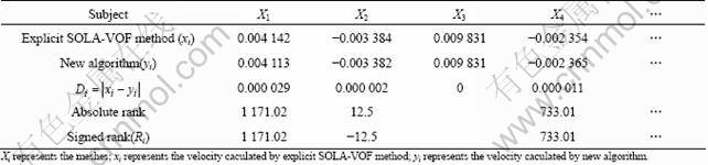
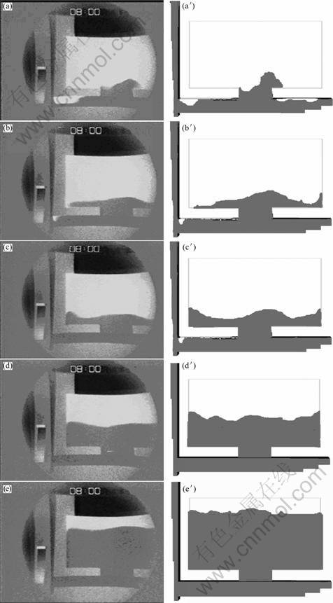
Fig. 2 Experiment results and simulation results of new algorithm in benchmark test: (a), (a′) 1.0 s; (b), (b′) 1.5 s; (c), (c′) 2.0 s;   (d), (d′) 2.5 s; (e), (e′) 3.0 s

Figure 2 illustrates both the experiment results and the simulation results of the new algorithm. It is clear that the simulation results agree well with the experiment results.

The new algorithm takes 601 s to complete the calculation and the explicit SOLA-VOF method takes 818 s, the calculating is reduced by 27%. It is true that the new algorithm calculates quickly than the SOLA-VOF method using the explicit difference method.

6 Conclusions

1) The new algorithm based on the projection method with the implicit finite difference technique can be used for calculating the filling process effectively.

2) The filling process of the same aluminum casting is calculated by the new algorithm based on the projection method with the implicit finite difference technique and the SOLA-VOF method using the explicit difference method. Analysis results show that the simulation results are unanimous between the new algorithm and the explicit SOLA-VOF method. The simulation results of the new algorithm are in good agreement with the experiment ones. It is obvious that the new algorithm is correct.

3) The new algorithm calculates more quickly than the explicit SOLA-VOF method. In this work, the new algorithm reduces calculating time by 27%.

References

[1] CHEN Ye, ZHAO Yu-hong, HOU hua. Numerical simulation for thermal flow filling process casting [J]. Transactions of Nonferrous Metals Society of China, 2006, 16(2): 214-218.

[2] WEN Gong-bi, CHEN Zuo-bin. Unsteady/steady numerical simulation of three-dimensional incompressible navier-stokes equations on artificial compressibility [J]. Applied Mathematics and Mechanics, 2004, 25(1): 53-65.

[3] HOU Hua, YANG Rui-feng. Study on stainless steel electrode based on dynamic aluminum liquid corrosion mechanism [J]. Journal of Environmental Sciences, 2008, 21: 170-173.

[4] XU Ying, WU Yue-bin, SUN De-xing. Theoretical research on flow characteristic of urban sewage [J]. Journal of Harbin Institute of Technology, 2010, 42(8): 1292-1296.

[5] OISHI C M, TOME M F, CUMINATO J A, McKEE S. An implicit technique for solving 3D low Reynolds number moving free surface flows [J]. Journal of Computational Physics, 2008, 227(16): 7446-7468.

[6] FERREIRA V G, KUROKAWA F A, OISHI C M, KAIBARA M K. Evaluation of bounded high order upwind scheme for 3D incompressible free surface flow computations [J]. Mathematics and Computers in Simulation, 2009, 79(6): 1895-1914.

[7] TOME M F, CASTELO A, FERREIRA V G, MCKEE S. A finite difference technique for solving the Oldroyd-B model for 3D-unsteady free surface flows [J]. Journal of Non-Newtonian Fluid Mechanics, 2008, 154(2): 179-206.

[8] TOME M F, MANGIAVACCHI N, CUMINATO J A, CASTELO A, MCKEE S. A finite difference technique for simulation unsteady viscoelastic free surface flows [J]. Journal of Non-Newtonian Fluid Mechanics, 2002, 106(2): 61-106.

[9] TOME M F, GROSSI L, CUMINATO J A, CASTELO A, MCKEE S, WALTERS K. Die-swell, splashing drop and a numerical technique for solving the Oldroyd-B model for axisymmetric free surface flows [J]. Journal of Non-Newtonian Fluid Mechanics, 2007, 141(2): 148-166.

[10] HOU Hua. Studies on numerical simulation for liquid-metal filling and solidification during casting process [D]. Saitama, Japan: College of Materials Science and Engineering, Saitama Institute of Technology, 2005: 23-69.

[11] DENARO F M. On the applications of the Helmholtz-Hodge decomposition in projection methods for incompressible flows with general boundary conditions, Int [J]. Numer Meth Fluids, 2003, 43(1): 43-69.

[12] HODGE W V D. The theory and applications of harmonic integrals [M]. Cambridge, UK: Cambridge University Press, 1952: 29-50.

[13] IKENO T, KAJISHIMA T. Finite-difference immersed boundary method consistent with wall conditions for incompressible turbulent flow simulations [J]. Journal of Computational Physics, 2007, 226(2): 1485-1508.

[14] MIRBAGHERI S M H, DADASHZADEH M, SERAJZADEH S, TAHERI A K, DAVAMI P. Modeling the effect of mould wall roughness on the melt flow simulation in casting process [J]. Applied Mathematical Modelling, 2004, 28(11): 933-956.

[15] MIRBAGHERI S M H, ESMAEILEIAN H, SERAJZADEH S, VARAHRAM N, DAVAMI P. Simulation of melt flow in coated mould cavity in the casting process [J]. Journal of Materials Processing Technology, 2003, 142(2): 493-507.

[16] PANG Sheng-yong, CHEN Li-liang, ZHANG Ming-yuan, YIN Ya-jun. Numerical simulation two phase flows of casting filling process using SOLA particle level set method [J]. Applied Mathematical Modelling, 2010, 34(12): 1-17.

[17] SIRRELL B, HOLLIDAY M, CAMPBELL J. Benchmark test [J]. Modeling of Casting, Welding and Advanced Solidification Processes Ⅶ, 1995, 48(3): 915-933.

[18] CONOVER W J. Practical nonparametric Statistics [M]. New York: Wiley Publishing, Inc, 2006: 194-207.

[19] PAPADATOS N. Intermediate order statistics with applications to nonparametric estimation [J]. Statistics and Probability Letters, 1995, 22(3): 231-238.

[20] BALAKRISHNAN N, TRIANTAFYLLOU I S, KOUTRAS M V. Nonparametric control charts based on runs and Wilcoxon-type rank-sum statistics [J]. Journal of Statistical Planning and Inference, 2010, 139(9): 3177-3192.

[21] CHOUDHURY J, SERFLING R J. Generalized order statistics, bahadur representations, and sequential nonparametric fixed-width confidence intervals [J]. Journal of Statistical Planning and Inference, 1988, 19(3): 269-282.

[22] GLEN MEEDEN. Noninformative nonparametric bayesian estimation of quantiles [J]. Statistics and Probability Letters, 1993, 16(2): 103-109.

基于投影法求解三维不可压缩粘性方程的新算法

牛晓峰¹, 梁 伟¹, 赵宇宏², 侯 华², 穆彦青², 黄志伟², 杨伟明²

1. 太原理工大学 材料科学与工程学院，太原 030024；

2. 中北大学 材料科学与工程学院，太原 030051

摘  要：提出一种新的基于投影法的隐式有限差分算法，用于计算速度场和压力。这种方法的特点是将计算区域根据雷诺数分成几个区域；对于远离壁面的区域，热金属流按牛顿流计算；对于贴近壁面的区域，热金属流按非牛顿流计算。通过非参数统计和实验的方法证明新算法的正确性。数值模拟结果表明，新算法的计算速度要快于基于SOLA-VOF法的显式有限差分方法。

关键词：隐式有限差分方法；三维不可压缩粘性方程；投影法；非参数统计

(Edited by FANG Jing-hua)

Foundation item: Project (50975263) supported by the National Natural Science Foundation of China; Project (2010081015) supported by International Cooperation Project of Shanxi Province, China; Project (2010-78) supported by the Scholarship Council in Shanxi province, China; Project (2010420120005) supported by Doctoral Fund of Ministry of Education of China

Corresponding author: HOU Hua; Tel: +86-351-3557006; E-mail: houhua@263.net; LIANG Wei; Tel: +86-351-6018398; E-mail: liangwky@126.com

DOI: 10.1016/S1003-6326(11)60937-0