J. Cent. South Univ. (2018) 25: 2219-2244

DOI: https://doi.org/10.1007/s11771-018-3909-2

Dynamic analysis, simulation, and control of a 6-DOF IRB-120 robot manipulator using sliding mode control and boundary layer method

Mojtaba HADI BARHAGHTALAB¹, Vahid MEIGOLI¹, Mohammad Reza GOLBAHAR HAGHIGHI², Seyyed Ahmad NAYERI³, Arash EBRAHIMI⁴

1. Department of Electrical Engineering, School of Engineering, Persian Gulf University, Bushehr 7516913817, Iran;

2. Department of Mechanical Engineering, School of Engineering, Persian Gulf University, Bushehr 7516913817, Iran;

3. Department of Communication, School of Electrical and Computer Engineering, Tehran University, Tehran 1417614418, Iran;

4. Institute of Electrical Power Engineering, Faculty of Computer Science and Electrical Engineering (IEF), Rostock University, Rostock 18059, Germany

Central South University Press and Springer-Verlag GmbH Germany, part of Springer Nature 2018

Abstract: Because of its ease of implementation, a linear PID controller is generally used to control robotic manipulators. Linear controllers cannot effectively cope with uncertainties and variations in the parameters; therefore, nonlinear controllers with robust performance which can cope with these are recommended. The sliding mode control (SMC) is a robust state feedback control method for nonlinear systems that, in addition having a simple design, efficiently overcomes uncertainties and disturbances in the system. It also has a very fast transient response that is desirable when controlling robotic manipulators. The most critical drawback to SMC is chattering in the control input signal. To solve this problem, in this study, SMC is used with a boundary layer (SMCBL) to eliminate the chattering and improve the performance of the system. The proposed SMCBL was compared with inverse dynamic control (IDC), a conventional nonlinear control method. The kinematic and dynamic equations of the IRB-120 robot manipulator were initially extracted completely and accurately, and then the control of the robot manipulator using SMC was evaluated. For validation, the proposed control method was implemented on a 6-DOF IRB-120 robot manipulator in the presence of uncertainties. The results were simulated, tested, and compared in the MATLAB/Simulink environment. To further validate our work, the results were tested and confirmed experimentally on an actual IRB-120 robot manipulator.

Key words: robot manipulator control; IRB-120 robot; sliding mode control; sliding mode control with boundary layer; inverse dynamic control

Cite this article as: Mojtaba HADI BARHAGHTALAB, Vahid MEIGOLI, Mohammad Reza GOLBAHAR HAGHIGHI, Seyyed Ahmad NAYERI, Arash EBRAHIMI. Dynamic analysis, simulation, and control of a 6-DOF IRB-120 robot manipulator using sliding mode control and boundary layer method [J]. Journal of Central South University, 2018, 25(9): 2219–2244. DOI: https://doi.org/10.1007/s11771-018-3909-2.

1 Introduction

Robots have been designed and built in different shapes and for different applications. It can be said that the most important and functional of these are robotic manipulators, which have been developed to imitate human hands. Industrial robotic manipulators were introduced in 1950 to replace humans in dangerous tasks and to increase productivity and improve quality. The transportation, welding, turnery, painting, assembly, and manufacture of parts are common tasks that robots have been designed to carry out [1].

Robots are more useful than human beings in these jobs for several reasons (e.g., safety, accuracy, speed, increase in generation power, and flexibility) and are used in costly, dangerous, repetitive, and tedious tasks in industry as well as in harsh environments such as space, underwater, and in nuclear reactors. Humans are responsible for guiding the robot to reach the desired goal, which includes planning the joint motion of a robot to produce the right paths and calculating and producing the joint torque to track these paths accurately.

When controlling the position and velocity of robotic manipulators, having knowledge of their position and velocity is important. In practice, however, disturbances affecting the manipulator, uncertainties in the model, mismatches in system parameters, and the existence of higher-order dynamics lead to changes in model parameters that can decrease proper control and cause system instability.

In recent decades, attention has been focused on controlling the movement of the robot manipulator. A variety of control methods and controllers have been implemented, each with its own advantages and disadvantages. The following control methods are examples: robust [2, 3], optimal [4, 5], adaptive [6, 7], linear PID [8, 9], intelligent (including neural networks and fuzzy control types I and II), nonlinear sliding mode controller (SMC), inverse dynamic controller (IDC), computed torque [10], and Lyapunov-based control methods [11, 12].

PI and PID linear controls are conventional control methods for robotic manipulators that are widely used in industry [13]. As is evident, linear controls are inefficient and subject to uncertainties, and do not exhibit appropriate and robust performance. The robust H-infinity (H_∞) control method is used in robot manipulator systems to debilitate external disturbances and make the system stable [14]. However, the robust control obtained from the H_∞ method usually belongs to a higher order that makes implementation complex. Several order reduction methods have been suggested to address problems in the controller. Because most of these methods have non- deterministic polynomial time hard (NP-hard)-type polynomial complexity, they demand a significant amount of computing time. On the other hand, although local methods are fast, they do not guarantee overall convergence of the system [15].

Neural networks have an innate ability to teach, learn, and estimate nonlinear functions with arbitrary precision. This feature in control is used to model complex processes and compensate for unstructured uncertainties [16]. However, it is inevitable that the learning process reduces transient operation when dealing with disturbances. For systems such as robot manipulators that are subject to uncertainties, information about the model is not used efficiently and degrades the performance of the system’s transient state.

In addition, the use of global activation functions and local learning methods create problems in conventional neural networks that include low speed in learning, probability of failure to reach an appropriate answer, and extreme sensitivity to initial network weights. The control of the manipulator position using neural networks has been addressed in several articles [17–20].

Because fuzzy control usually does not need a mathematical model of the control system, it can be applied easily and performs well in systems that are complex, ill defined, nonlinear, and time varying. The primary advantage of fuzzy control is the use of human knowledge (expert experience), which is part of the process of control [21]. Its biggest disadvantage is weakness in investigating the theory of fuzzy controller stability. In fact, fuzzy control cannot guarantee the stability of a system because it lacks an explicit mathematical model to show it. For example, SONG et al [22] used a fuzzy control method to control the computed torque of manipulators. Moreover, PILTAN et al [23] applied a fuzzy logic controller for a PUMA robot manipulator.

An inverse dynamic controller (IDC) with integral action [24, 25] is a nonlinear controller having the ability to delete disturbances and other types of uncertainties from the system to some extent. Because it is inherently nonlinear, IDC is a robust controller for which variations in robot parameters do not affect performance. In order to track the desired trajectory more accurately, the IDC controller is capable of disturbance rejection. This controller has two major faults in the control of robotic manipulators. One is that the transient state response of the system is insufficient, and the overall response of the system is very slow. Another is that the controller increases the tracking errors of the system. For example, BABAIASL et al [26] and GHOBAKHLOO et al [27] applied an IDC to robotic manipulators.

The sliding mode theory was first proposed by researchers in the Soviet Union in 1950. A sliding mode control (SMC) differs from a simple relay controller because it relies on high-speed switching of control values and can be changed instantaneously from one structure to another, making it appropriate for controlling robotic manipulators. In the current manipulator, linear PI and PID controllers are used because they can be easily implemented, but a linear controller is not effective enough when coping with uncertainties. Hence, the use of nonlinear controllers, which can cope with uncertainties, is recommended in order to achieve appropriate and robust performance.

An SMC [28] is a robust state feedback control method for nonlinear systems that has a simple design and is efficient and practical in overcoming structured uncertainties, nonstructured uncertainties, and external disturbances of the system. It also has a fast transient response and appears to be a highly desirable method of controlling robotic manipulators. However, its control signal is discontinuous and produces adverse chattering phenomena [28] that may stimulate the high- frequency dynamics of system and, in the worst case, cause system instability.

In this study, to solve the problem of chattering, an SMC with a boundary layer is used. In addition to eliminating chattering in the SMC, it improves system performance. However, the use of this method can slightly increase the steady-state error of the system. To solve the problem of chattering, the use of a higher-order SMC or fuzzy SMC is customary. The former increases the computational complexity of the system, which is undesirable, and the latter causes an undesirable transient response in the system, makes it slow, and also creates a problem with the investigation of the theory of fuzzy controller stability.

PILTAN et al [29] used an SMC to control a PUMA-560 robot in a MATLAB/Simulink environment. CORRADINI et al [30, 31], CAPISANI et al [32–34], and JIN et al [35] implemented SMC on industrial and laboratory robotic manipulators and tested them experimentally. Recently, BABAIASL et al [36], with the help of our colleagues, used an SMC to control an exoskeleton robot designed for upper-limb rehabilitation of the human body. The results were simulated and tested in a MATLAB/ Simulink environment. NEKOUKAR et al [37] used a fuzzy-adaptive estimator to estimate the system dynamics and a nonlinear SMC based on the estimated dynamics to control the dynamic system. The efficiency of this method was demonstrated on a robot manipulator system. Moreover, different types of fuzzy-SMC methods were applied previously to manipulators [38–42].

SOLTANPOUR et al [43, 44] presented a robust fuzzy SMC and examined a robust fuzzy-adaptive SMC for tracking a 2-DOF robot manipulator in the presence of uncertainties. An optimal fuzzy SMC approach was used [45], and VEYSI et al [46] designed a self-adaptive optimal fuzzy SMC for tracking a 2-DOF robot manipulator in the presence of uncertainties, which led to successful results.

Adaptive neuro-fuzzy control has been implemented in industrial and laboratory robotic manipulators in previous studies [47–50]. WANG et al [51] and SUN et al [52] introduced a combined SMC and neural network control method for controlling robot manipulators. WAI et al [53, 54] used a combined SMC and neuro-fuzzy control method to control a 2-link robot manipulator. HU et al [55] used a combined SMC and neural network method with a fuzzy supervisor to control a 2-link robot manipulator.

KHOOBAN et al [56] introduced an optimal hybrid control approach called the optimal general type-2 fuzzy sliding mode to control electric vehicles. This interesting idea can be used to control a robot manipulator.

In a recent paper [57], we combined SMC and an adaptive neuro-fuzzy network (ANFIS) with the fuzzy supervisor method to control the first three links of an IRB-120 robot. Note that this was not a mature work and contained deficiencies and faults that we are trying to address to improve the control method. The results of that research will be presented in the form of a new article in the near future.

In the current study, SMC without a boundary layer and with a boundary layer was applied to a 6-DOF IRB-120 robot manipulator in the presence of uncertainties. The results were simulated, tested, and compared in a MATLAB/Simulink environment. For further validation, the results were also tested and confirmed experimentally on an actual IRB-120 robot manipulator. The main contribution of the current study and its unique features are as follows:

This marks that a controller has been designed for an IRB-120 industrial robot manipulator for which all of the kinematic and dynamic equations were extracted. The current study can be the beginning of more extensive studies on the design of controllers of IRB-120 robot manipulators, instead of the PUMA-560 robot on which most studies have concentrated up to now.

The problem of chattering in sliding mode controllers has been solved with the introduction of a simple control method and tiny modifications to the control input signal equation to obtain relatively suitable results. In conventional methods, fuzzy control and adaptive control or neural networks (combined with the SMC) have been used in place of SMC to solve the problem of chattering. The use of each method has its own problems and complexities. Some of these problems are as follows.

The main problem of the use of fuzzy control besides the SMC in Refs. [37–46] and [56, 57] was addressed as a lack of an explicit mathematical model. In addition, the formulation and estimation of the disturbances along with the system dynamics are difficult. The lack of an explicit mathematical model leads to the inability to investigate and guarantee the stability of a fuzzy control system. In other words, there is an inherent weakness in theoretical investigations of fuzzy controller stability.

The main problem in the use of adaptive control besides the SMC in Refs. [37, 44, 46], and [47–50] has been explored. This problem is related to the application of adaptive parameters in the adaptive update rules, which requires more inputs and parameters in these controllers. As a result, the computation volume increases, which is not optimal.

The primary problem of the use of neural networks besides the SMC in Refs. [47–54, 57] has been stated to be learning by the neural network. Learning by neural networks causes the transient response of the system to slow and become inappropriate. This reduces the convergence rate of the error, which is of great importance when controlling robotic manipulators.

In general, the main advantages of the proposed control method as compared to other methods are the application of SMC, its simplicity, the smoothness of the control scheme, and the absence of the problems and complexities mentioned above. Despite the simplicity of the structure in the proposed model, the results obtained are relatively similar to those of conventional methods with complex structures.

The structure of the remainder of the paper is as follows: Section 2 describes the structure and mechanics of an industrial 6-DOF IRB-120 robot manipulator. Section 3 extracts the direct kinematics of the robot manipulator, a Jacobian matrix, and its dynamic equations of motion. Section 4 explains how to design controllers and implement them on the IRB-120 manipulator robot. It first introduces the comparative control method (IDC) and provides the results of simulating IDC on the IRB-120 robot manipulator. It then introduces the proposed control method, SMC, without and with a boundary layer, and compares the simulation results of this method with the IDC method.Section 5 discusses experimental results, and Section 6 presents the conclusions. Appendix 1 shows the table of notations and symbols used in the equations in this study.

2 Characteristics and mechanical design of 6-DOF robot manipulator

A sliding mode controller for an IRB-120 industrial robot manipulator is presented as an example of a 6-DOF industrial robotic manipulator and is used to simulate, test, and compare the results. This section introduces the structure and mechanics of an IRB-120 manipulator. Section 3 then discusses the kinematics and dynamic equations of the robot used in its control.

2.1 Structure of IRB-120 robot manipulator

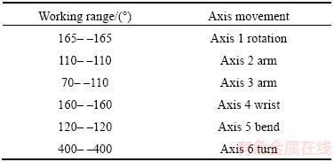
In October 2009, the smallest multipurpose industrial robot, IRB-120, was presented by the ABB company. A robotic manipulator with 6 DOF has all the capabilities and advanced design features of ABB’s large robot, yet it is very lightweight and cost effective. It has a mass of only 25 kg, and it has accessibility to 580 mm and the ability to reach 112 mm below its own base. It has a rotating arm structure and spherical wrist structure, and a structure similar to that of the PUMA-560 robot. The important aspects of the IRB-120 robot and range of changes in each joint axis are shown in Figure 1 and Table 1, respectively.

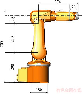
Figure 1 Important aspects of IRB-120 robot (Unit: mm)

Table 1 Range of changes in joint axes of IRB-120 robot

2.2 Mechanical design of IRB-120 robot manipulator in SolidWorks software

To extract the dynamic equations of the IRB-120 robot, the center of mass and moment of inertia of each link of the robot are required. Because there was no precise information about the center of mass or moment of inertia, the model was simulated in SolidWorks software environment to obtain them. Information about the center of mass and moment of inertia were derived from output of SolidWorks (in the part “mass properties”). A schematic model of the robot simulated in SolidWorks is shown in Figure 2.

Figure 2 Schematic of IRB-120 robot simulated in SolidWorks

This robot stimulation model is formed from seven segments: six links and one fixed holder base. Because all the joints of the IRB-120 robot are revolute, a 6-DOF revolute was used.

Table 2 lists the general features of the robot and the dynamic specifications of its links. This table contains information such as the length, weight, and moment of inertia around the center of mass of each link and the center of mass of each link relative to the reference coordinate system.

3 Kinematic and dynamic analysis of 6-DOF IRB-120 robot manipulator

In this section, the kinematic and dynamic equations of the 6-DOF robot used in the controller are obtained. It is essential to have a dynamic model to understand and design a robot manipulator controller.

3.1 Direct kinematics of robot manipulator

Kinematics is the science of motion, regardless of its creative forces. To obtain the kinematic equations of a robot mechanism, each link is considered as a rigid body to describe the relationship between the two neighboring joint axes in the manipulator. The joint axes in space are defined by lines. To produce robot kinematic equations, a simplified kinematic model of the robot first must be obtained [58]. Figure 3 shows a simple kinematic model of the IRB-120 robot along with the frames attached to it.

Table 2 Dynamic characteristics of all components of IRB-120 robot

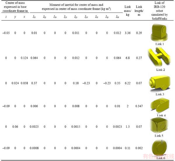
Figure 4 shows the Denavit-Hartenberg (D-H) parameters [24, 25] for the IRB-120. The D-H parameters for the IRB-120 listed in Table 3 are a_i (link length), α_i (link twist), d_i (link offset), and θ_i (joint angle).

Figure 5 is a schematic view of the coordinate systems, joints, joint angles, and centers of mass of the IRB-120 robot manipulator. Because all joints of the IRB-120 robot are revolute, the robot mechanism is 6-R (revolute). In the three joints of the arm, the axes of the second and third joints are parallel to one another and are vertical to the first joint. In the three axes of the ankle, the axes of the fourth and fifth joints are vertical to each other, and the fourth joint is parallel to the sixth joint (Figures 3 and 5).

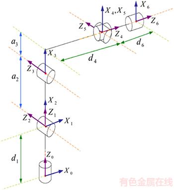
Figure 3 Simple kinematic model of IRB-120 robot

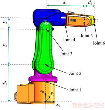
Figure 4 D-H parameters of IRB-120 robot

Table 3 IRB-120 robot D-H parameters

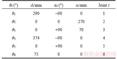
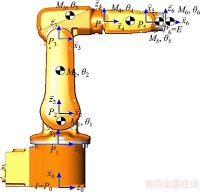
Figure 5 Schematic of coordinate systems, joints, joint angles, and centers of mass of IRB-120 robot

Given the parameters in Table 3, the transformation matrices for the robot links are obtained as follows [24, 25]:

                      (1)

The homogeneous overall conversion matrix of the robot that connects the end-effector coordinates to the base coordinates is obtained as follows:

        (2)

where

 (3)

where c_i and s_i are the representative of cosθ_i and sinθ_i, respectively. According to Table 3, these are d₁=290 mm, d₄=302 mm, d₆=72 mm, a₂=270 mm and a₃=70 mm.

These equations are actually the kinematic equations of the IRB-120 robot. The position and orientation of the robot end-effector can be obtained by having the θ_i values.

3.2 Jacobian matrix of robot

In robotics, the Jacobian matrix represents the relationship between the end-effector velocity and the velocity of the joints, as follows:

                              (4)

For a 6-link robot, v_e is a 6×1 vector of the linear and angular velocity of the end-effector, and is a 6×1 vector of the joint velocities. J is the robot Jacobian matrix and is a size 6×1 matrix. Because all joints of an IRB-120 robot are revolute, the Jacobian matrix of the robot can be calculated as follows [29, 30]:

 (5)

where z₁, z₂, z₃, z₄, z₅ are the first three elements of the third column of the matrixes obtained by successive multiplication of Eq. (1) matrixes, respectively, and O₁, O₂, O₃, O₄, O₅, O₆ are the first three elements of the fourth column of the matrixes, respectively, obtained from the following relations as

 (6)

The Jacobian matrix of the 6-link IRB-120 robot is shown below. The robot dynamic equations can be obtained using this equation as

 (7)

where v_i is the linear velocity of the center of mass of the ith link; ω_i is the angular velocity of the center of mass of the ith link; J_vi and J_ωi are the upper and lower halves of the Jacobian matrix and depend upon the linear and angular velocities, and c_i and s_i are representative of cosθ_i and sinθ_i, respectively.

The unknown values of the elements in this Jacobian matrix are shown in Eq. (8). The Jacobian matrix of the robot was calculated once manually and implemented and validated once in the MATLAB/Simulink environment. In accordance with Eqs. (5) and (6):

     (8)

3.3 Dynamics of robot manipulator

Robot dynamics examines robot motion as related to the forces and torques that have created this motion. Here, the Lagrange-Euler equations [24, 25] are used to obtain the dynamic equations of the robot. An advantage of this method is that it is simple and clear.

Because the manual extraction of the dynamic equations of a 6-link robot, given the volume of its Jacobian matrix, is difficult and complex and requires many time-consuming calculations, only the three primary joints of the robot arm were considered and three final joints of the robot wrist were assumed to be constant such that q₄=q₅=q₆=0. The equations were derived only for the three primary links out of the total of six links in the robot dynamic equations.

Note: It should also be noted that the facilities provided by MATLAB allowed for the complex and lengthy dynamic calculation for every six links using “symbolic variables.”

The 3-link manipulator with revolute joints is shown in Figure 6. In the figure, q_i shows the position or angle of the ith joint (q₁, q₂, q₃ are the same as joint angles θ₁, θ₂, θ₃ in Table 2); m_i is the mass of the ith ink; I_i is the inertial tensor matrix in the center of mass of the ith link that was defined in Eq. (9); l_i is the distance between the previous joint and the center of mass of the ith link; d₁, a₂, a₃ show the lengths of each link. The values of these parameters for the IRB-120 robot are listed in Tables 2 and 3.

i=1, 2, 3            (9)

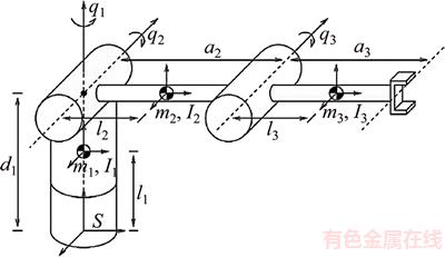
Figure 6 Schematic of 3-link manipulator with revolute joints

As mentioned, the Lagrange-Euler method was used to obtain the dynamic equations of the robot. In this method, the dynamic equations can be expressed in the following matrix form as [25]:

                (10)

For a 3-link robot, D(q) is a 3×3 symmetric positive definite matrix called an inertial matrix and is obtained using Eq. (11).is a 3×3 matrix related to the Coriolis and centrifugal terms obtained using Eq. (12), and G(q) is a 3×1 matrix related to the gravity term obtained using Eq. (13). In addition, τ is a 3×1 matrix related to the robot torque of the joints, and are 3×1 matrices that are respectively related to the position, velocity, and acceleration of the robot’s joints.

         (11)

where J_vi and J_ωi depend on the linear and angular velocities of the center of mass of the ith link, and R_i is the homogeneous rotation transformation matrix of the ith link.

            (12)

where C_kj are the elements of thematrix, c_ijk are called the Christoffel symbols ,and d_ij are elements of the D(q) matrix.

                            (13)

                        (14)

In Eq. (13), g_k(q) are gravity elements. In Eq. (14), g₀ is a gravitational constant, 9.8 m/s² and h_ci(q) is the height of the ith link center of mass.

The derivation of robot dynamic equations requires a Jacobian matrix. In this case, the Jacobian matrix for the 3-link manipulator can be calculated using Eq. (15) [24, 25] as

 (15)

where c_i and s_i are representative of cosθ_i and sinθ_i, respectively, and c₂₃c₂c₃–s₂s₃ and s₂₃s₂c₃+ c₂s₃ are defined contractually.

Using Eq. (10), dynamic equations are obtained in the form of the following matrix for a 3-link manipulator of an IRB-120 robot as

                         (16)

where each C_kj element is defined as the sum of the Christoffel symbols inform, and the values of the passive elements of each matrix D(q), and G(q) are [24, 25] as follows.

According to Eq. (11), we have

                (17)

According to Eq. (12), we have

     (18)

In addition, according to Eqs. (13) and (14) and assuming a₁=0, a₂=270, a₃=70 in Table 3, we have

                     (19)

In the above equation, c₁₂c(q₁+q₂), c₁₂₃c(q₁+ q₂+q₃), and l_i is the distance between the center of the mass of the ith link of the robot and the predecessor joint.

The dynamic equations of the IRB-120 robot were calculated once manually and were implemented and validated once in the Simulink/ MATLAB environment. The dynamic calculations of the robot for every six links were done in MATLAB using symbolic variables.

4 Controller design for IRB-120 robot manipulator

Robot manipulators are inherently nonlinear systems. As is known, the linear PID control method is not appropriate for controlling such systems as it lacks sufficient effectiveness and robustness to the uncertainties and disturbances in the system. Therefore, to control a robot manipulator, it is necessary to adopt nonlinear control methods to overcome uncertainties and disturbances and to resist variations in parameters. This is why the IDC method, a conventional nonlinear method, was used to compare the results with those of the proposed SMC method.

This section first explains the theory behind the comparative control method (IDC). It also provides the results of simulating this method on an IRB-120 robot. It then explains the theory of the SMC method and compares the results of the simulation with those obtained from the IDC method.

4.1 Implementation of inverse dynamics controller (IDC) on IRB-120 robot manipulator

This section explains the design of the comparative control method, IDC, with integral action [24, 25], and implements it on the IRB-120 robot manipulator. IDC is a nonlinear controller that can remove disturbances and other types of uncertainties from the system to some extent. Because it is inherently nonlinear, IDC is a robust controller for which variations in robot parameters do not affect performance. In order to track the desired trajectory more accurately and completely, the controller should be capable of removing disturbances.

This study assumed constant and bounded disturbances. The uncertainties of the system were modeled as constant and bounded disturbances. If d is the torque caused by uncertainties and disturbances in the system, and τ is the input torque of the robot joints, considering Eq. (10), the dynamic model of the system can be stated as follows [24, 25]:

                 (20)

where and |d(t)|≤d_m.

The proposed control action for the system is suggested as follows:

                 (21)

 (22)

where error vector e(t) and its first and second derivatives are defined as

       (23)

In the above system, the aim of control is for the q(t) output of the system to track the desired q_d(t) bounded output.

Substituting the results of Eqs. (21) and (22) into Eq. (20) and considering Eq. (23) produces:

      (24)

        (25)

where K_P, K_D, K_I are the proportional coefficients, derivative coefficients, and integral coefficients, respectively. They are stated as three positive definite matrixes in Eq. (25). Note that in IDC, the integral term has a disturbance rejection property.

Figure 7 shows a block diagram of the closed- loop control system of the IRB-120 robot for the IDC.

The simulation results of the IDC on the IRB-120 robot manipulator were derived using MATLAB. To this end, the values of k_p, k_d, k_i were set at k_p=20, k_d=10, k_i=10. The duration of simulation was set at 10 s, and as stated, this study assumed a constant and bounded input disturbance signal.

Figure 8 shows the step response of the system, position tracking error, velocity tracking error, and control input torque of the simulated IDC at the 1 to 6 joints of the IRB-120 robot. Figures 8(a) to (f) show that the transient state response of the system was very slow. In addition, there was a steady-state error in the system (e_ss≠0). This means that as the length of the tracking error decreased over time, it did not fall to absolute zero (Figures 8(g) to (r)). Therefore, the controller was faulty in terms of the above two problems, and the faults needed to be eliminated. For the proposed controller, the faults were eliminated as much as possible.

4.2 Implementation of sliding mode controller (SMC) on IRB-120 robot manipulator

The sliding mode controller (SMC) is a robust state feedback control method for nonlinear systems with structural changes to achieve optimal performance [28]. In addition to having a simple design, SMC is efficient and practical in overcoming the structured and unstructured uncertainties and external disturbances of the system. When designing SMC, it is assumed that the control can be changed instantaneously from one structure to another.

Figure 7 Block diagram of closed-loop control system of IRB-120 robot for IDC

Figure 8 IDC at 1 to 6 joints of IRB-120 robot:

In practical systems, however, computational delays in the timing of control signal computations and restrictions on operators mean momentary change is not possible. A chattering phenomenon arises as a result. To address chattering, higher- order SMC or the use of boundary layers is common. The former increases the computational complexity of the system, which is not desirable. In the following, the use of SMC to control the robot manipulator will be explained [28].

In SMC, the dynamic equations of the robot can be used to control it. Using Lagrange-Euler equations in the form of a matrix, the dynamic equations can be expressed as shown in Eq. (10). This equation can be rewritten as

            (26)

in which and |d(t)|≤d_m, where d(t) is the torque caused by limited uncertainties and disturbances in the system, and d_m is a positive constant.

To design the SMC, the dynamic equation of the robot is rewritten as

        (27)

where is the state vector of the system; is the system output that represents the position of the robot joints, and τ(t) is the control input torque related to the robot joint torques. To design the control input, it is assumed that the states of the system are measurable. Error equations for the system in Eq. (27) are defined as

                      (28)

where is the position tracking error, and is the velocity tracking error. In the control target of the system, the q(t) output tracks the q_d(t) bounded desired output. For each degree of freedom, the sliding surface is defined as

                (29)

where n is the number of system DOFs, and λ_i are constant and positive values. Sliding surface s_i is a weighted sum of the position and velocity error. By defining s_i as above, the second-order q_d vector tracking problem with n DOF becomes a n-to-S first-order stabilization problem. For this, a vector composed of n sliding surfaces is defined as

                     (30)

In order for the tracking error to fall to zero for the control target , must be true. For this purpose, according to Eq. (29). This is equivalent to remaining on the S(t) sliding surface for t>0 times. For vector S to be kept at zero, the control input must be available such that

                        (31)

where η is a positive constant.

The above condition is called a sliding condition, and it means that the square of the distance to the sliding surface for all state trajectories declines. This is shown schematically in Figure 9. If this condition is established, starting from nonzero initial conditions, the state trajectories in a time of less than reach the time-varying sliding surface. Once placed on the sliding surface, the tracking error exponentially falls to zero [28]. This is shown schematically in Figure 10.

For a robot manipulator system, the τ(t) control input torque should be designed such that the output can track an optimal path. Moreover, the tracking error and all its derivatives go toward zero. The sliding surface and its derivative for a robot manipulator system are

Figure 9 Schematic representation of sliding condition

Figure 10 Schematic representation of sliding mode for second-order system

  (32)

where Λ is an eigenvalue matrix that is diagonal with positive elements for λ_i.

In the sliding phase, S(t)=0,and τ(t) are designed to maintain the system on the sliding surface. In this case, the τ(t) control input torque can be obtained as

       (33)

In a closing phase in which S(t)≠0, τ(t) is designed such that the conditions required to reach sliding surface are satisfied. To do this, consider the Lyapunov function as

                             (34)

which is a continuous and positive definite function. Its derivative can be obtained as

                               (35)

By calculating as shown in Eq. (36), it can be shown that Eq. (35) is negative and Eq. (34) descends, and the conditions of sliding surface are satisfied:

                (36)

where K is a gain control matrix that is diagonal to the positive elements of k_i and sign(S) is the sign function. Substituting Eq. (36) into Eq. (32) produces

    (37)

In this case, the τ(t) control input torque can be obtained as follows:

 (38)

In Eq. (38), K must be set to a value that will satisfy the sliding condition as

                             (39)

In the design of the SMC, the control input torque was obtained such that all signals are limited and bounded. In these relations, the feedback control law was designed to meet the sliding condition. To cope with model uncertainties and disturbances, the control signal was discontinuous in the vicinity of S. Its implementation in operational systems did not produce a desirable response and caused chattering in the control input of system. This is shown in Figure 11.

In general, chattering is an undesirable phenomenon that stimulates a system’s unmodeled high-frequency dynamics. In the worst case, it also causes system instability. It can be said that because of the discontinuous control signal created around the sliding surface that satisfies the sliding condition, the SMC is a robust controller. However, because of the discontinuous term, high-frequency oscillations are created in the controller input, and these oscillations are known as chattering [28].

To reduce chattering, the control input can be smoothed and softened by defining a boundary layer around the sliding surface [28]. The sliding surface from the control input signal can be calculated as shown previously, but the method of calculating the control input signal changes. For example, in control, the input torque τ(t), sat(S/φ) can be used instead of sign(S) in which φ is the boundary layer thickness. In this case, the control input torque is as follows:

 (40)

A schematic representation of the control input signal calculation considering the boundary layer is shown in Figure 12.

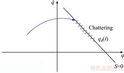
Figure 11 Schematic representation of chattering in system

Chattering can be avoided by smoothing the discontinuity of the control input signal in a thin boundary layer neighboring the switching surface, as follows:

              (41)

In Figure 12, is the equivalent control input obtained from and u is the control input τ(t) and is defined as

            (42)

Figure 13 shows a block diagram of the control system of the IRB-120 robot manipulator using the SMC. In addition, to better understand the proposed control method, the procedure of the proposed control is shown in Algorithm 1.

The simulation results for applying the SMC to the IRB-120 robot manipulator system are presented using MATLAB. First, the system response is offered using a simple SMC, and this response is improved using a boundary layer. In Eqs. (32), (36), and (38), control parameters λ_i and k_i are optimized using a primary optimization algorithm (in this case, a genetic algorithm or GA). The cost function of the GA is defined in Eq. (43). To minimize this cost function, the control parameters were obtained as shown in Eq. (44). Appendix 2 provides further explanations on how the optimized control parameters are obtained from the defined cost function for the GA.

          (43)

   (44)

Algorithm 1: Procedure of proposed control

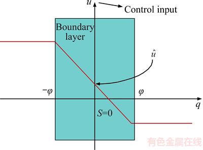
Figure 12 Schematic representation of control input signal calculation considering boundary layer

1. Definition of sliding surface To track, define the sliding surface as

2. Obtaining equivalent control input

To obtain equivalent control input differentiate sliding surface S and set it to zero . Then can be obtained as

3. Obtaining total control input u

To satisfy the sliding condition in Eq. (39), a discontinuous term must be added to across sliding surface S=0. The total control input u [the same control input τ(t) in Eq. (38)] can be obtained as

4. Removing chattering

To reduce chattering, smoother functions such as or can be used instead of sign function sign(S). Then, u can be obtained as

5. Selection of control parameter K

Control parameter K (in the above equations) should be selected to guarantee sliding condition

6. Applying control input u to plant

Control input u can be applied to the plant, the IRB-120 robot manipulator in this case, and output q can be obtained.

7. Comparison of output q and desirable output q_d

Then output q can be compared with desirable output q_d using state feedback. If skip to the end; otherwise, return to step 1 and repeat the steps.

In Eq. (43), β is the tuning parameter and is equal to 0.5, and e is the exponential function. M, e_ss, t_r, and t_s are the overshoot average, steady-state error, rise time, and settling time, respectively, for each joint of the robot. Note that the cost function of Eq. (43) was selected for the GA because the step response of the system is in the form of the step response of a first-order system, as shown in the simulation results in Figures 15 and 16. M, t_r, and t_s are the transient response specifications of the system, and e_ss is the steady-state response specifications and accuracy of the system.

For the cost function in Eq. (43), the first term is for the steady-state response (sliding phase:

and the second term is the transient state response (closing phase: As the cost function of Eq. (41) is optimized, the specifications of the steady-state and transient state response of the system are optimized. In this case, the best optimal and ideal step responses were generated in the simulation results. (Because the proposed system is a first-order system and there is no overshoot in the step response, the specification of M in Eq.(43) was removed.)In Eq. (40), in order to simulate a sliding mode controller with a boundary layer (SMCBL), the function was used to approximate saturation function sat(S/φ) in which z is obtained using the basic search algorithm. The control input torque can be obtained as follows:

                      (45)

Figure 14 shows the simulated total disturbance signal of system d(t) in the form of steps. This disturbance may indicate torque applied to the joints of the robot caused by structured uncertainties, unstructured uncertainties, or external disturbances in the system. Note that the uncertainties considered in the current study were divided into two parts.

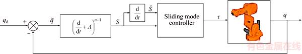
Figure 13 Block diagram of IRB-120 robot control system using sliding mode controller

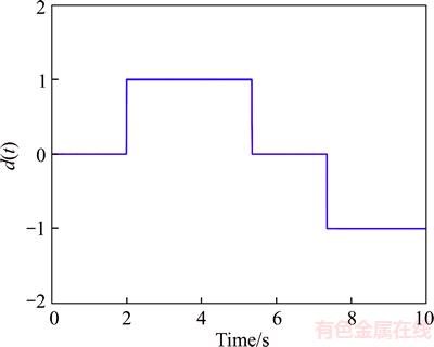
Figure 14 Simulated disturbance signal applied to each robot joint

Structured uncertainties (parametric uncertainties) indicate changes in the parameters of the robot links. Unstructured uncertainties include unknown external disturbances, unmodeled dynamics, and friction between the robot links. All of these are considered to be system uncertainties or system disturbances and are denoted as d(t) in this work.

Note that all simulations took place in real time so that chattering caused by computational delays at the time of input signal calculation is considered in the SMC. Moreover, the sampling time was set to T_s=0.01 s in the discrete-time sliding mode system.

Figure 15 shows the step response of the system, position tracking error, velocity tracking error, and control input torque of the simulated ordinary SMC at the 1 to 6 joints of the IRB-120 robot. As seen in Figure 15, the reference input tracking performed well, and the system had no steady-state error (e_ss=0) (Figures 15(g) to (r)). However, the chattering of the input signal was high (Figures 15(s) to (x)). It can also be seen that the transient response of the system was convenient and fast (Figures 15(a) to (f)). In order to apply the system, the input signal chattering must be removed because practical actuators are unable to apply a signal with this level of chattering. A convenient method for this is the use of an SMCBL.

Figure 16 shows the step response of the system, position tracking error, velocity tracking error, and control input torque of the simulated SMCBL at the 1 to 6 joints of the IRB-120 robot. As seen in Figure 16, with the use of SMC, the control input signal had chattering that would stimulate the unmodeled high-frequency dynamics of the system and could cause system instability (Figures 15(s) to (x)).

When SMCBL was used, the control input signal chattering disappeared, and the control input signal became smoother and softer. This signal was acceptable as a control input both theoretically and practically (Figures 16(s) to (x)). As shown in Figures 16(a) to (r), the system response was somewhat slow, and its tracking error increased slightly compared to the SMC without a boundary layer. This problem was negligible when compared to the elimination of chattering in the control input signal.

The simulation results of the SMCBL (Figure 16) were compared with those of a comparable controller (IDC, Figure 8). It was revealed that the step response of the SMCBL controller (Figures 16(a) to (f)] was more appropriate and faster than that of the IDC controller (Figures 8(a) to (f)]. In addition, the tracking error of the SMCBL controller (Figures 16(g) to (r)) decreased compared to that of IDC controller (Figures 8(g) to (r)).

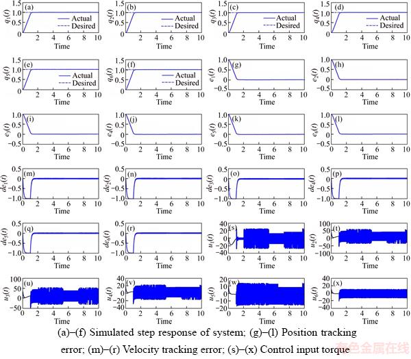
Figure 15 Ordinary SMC at 1 to 6 joints of robot:

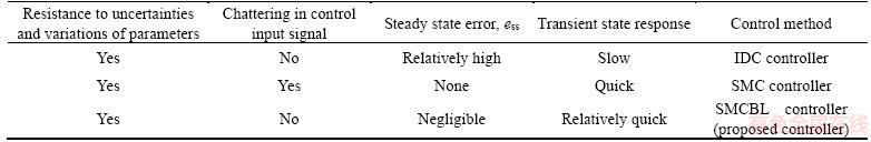
Table 4 briefly compares the SMCBL with the ordinary SMC and the IDC controller. Based on Table 4 and the simulation results, it can be argued that the SMCBL is more advantageous than the other controllers in terms of the transient state response, tracking error, and elimination of input signal chattering, and is a sufficient controller for the IRB-120 robot manipulator.

To demonstrate the stability and robustness of the proposed control method, the convergence curve of the proposed method is provided separately. In order to better show the convergence of the system output signal, instead of responding to the step input, the system response to the sinusoidal input was used. For this simulation, a desirable sinusoidal trajectory q_d was considered in the form of Eq. (46), and then system output q was measured using desirable trajectory q_d as

                       (46)

Figure 17 shows that for all six links of the IRB-120 robot manipulator, q of the system reached desirable trajectory q_d in less than 2 s and converged with it. Therefore, the stability (global asymptotical stability) of the proposed control method was guaranteed in a closed-circuit system and in the presence of uncertainties and disturbances in the system.

Note: The mathematical proof of the global asymptotical stability of a classic SMC in the presence of system uncertainties was provided by SOLTANPOUR et al [44]. This proof can be extended to the proposed control method; thus, it is not necessary need to repeat it for our control method.

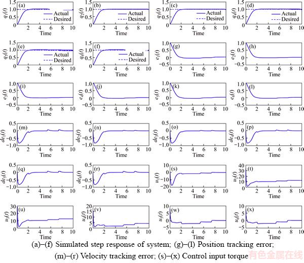
Figure 16 SMCBL at 1 to 6 joints of robot:

Table 4 Comparison of SMCBL with SMC and IDC controllers

5 Experimental results for proposed SMC controller

To further validate the current work, the results were tested experimentally on a real IRB-120 robot manipulator. The SMC was tested on a real IRB-120 robot manipulator in a laboratory environment, and the accuracy of simulation results was verified. As expected, the experimental results were obtained with an acceptable margin of error and confirmed the results obtained from the simulation.

Figure 18 is a photograph of the IRB-120 robot manipulator used with a practical control system that includes a three-phase voltage power supply (200–600 V, 50–60 Hz) that generates DC servomotor power to each robot joint. It includes a DC motor drive system that controls the position of each joint of the robot. It also includes a digital signal processor (DSP) module designed to apply control schemes to the robot manipulator and data by exchanging control commands.

The performance of the practical control system is as follows: first, control commands are transferred via a Notebook to the DSP module.

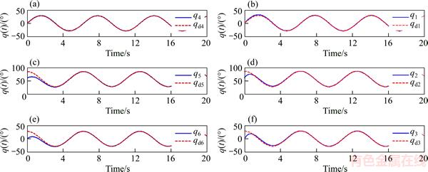
Figure 17 Simulated sinusoidal desirable trajectory tracking by system output for proposed controller at joints 1 to 6 of IRB-120 robot

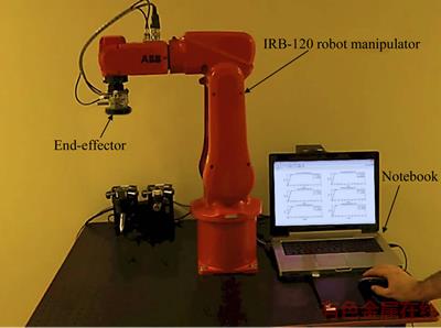
Figure 18 Photograph of IRB-120 robot manipulator in laboratory environment

These are then sent from the DSP module to the DC motor drive system, and from there are applied to the DC servomotor for each joint to control its position.

In a practical control system, implementation of control laws is done in real-time, and input signal chattering occurs naturally because of computational delays and restrictions on the operators. Here, a T_s=0.01 s sampling time was used in the practical discrete-time control system.

Figure 17 shows the SMC applied to a real IRB-120 robot manipulator in a laboratory environment. As expected, the experimental results obtained an acceptable margin of error similar to the results of the simulation in MATLAB. Figure 19 shows the application of the step input to each of robot joint, and the step response obtained for the ordinary SMC and SMCBL.

As can be seen, the step response of both the SMC and SMCBL controllers was relatively good. Although the response of SMCBL was slightly slower than that of SMC, this problem is negligible compared to the advantage of eliminating the chattering. Figure 20 shows the experimental control input torques of the SMCBL at joints 1 to 6 of the robot. The experimental results confirm the results of the simulation.

6 Conclusions

This paper presented dynamic analysis, simulation, and control of a 6-DOF IRB-120 robot manipulator in the presence of uncertainties using SMCBL. An investigation of the results of a simulation in MATLAB and the experimental results confirmed the performance and suitability of the proposed control method when compared with conventional methods including IDC (Table 4).

Nonlinear SMC is a sufficient replacement for conventional linear PID controllers in robotic manipulators. In addition to having a simple design, nonlinear SMC is efficient and practical in overcoming uncertainties and disturbances in a system. Moreover, it has a very fast transient state response, which is highly desirable when for controlling the robot manipulator. However, the biggest shortcoming of this method is the occurrence of chattering in the control input signal, which causes high-frequency oscillations in the system input and can result in system instability.

The SMCBL method was proposed to solve the chattering problem in SMC. In addition to eliminating the chattering, this method increases the efficiency of the system. The SMCBL smoothes the control input signal by defining a boundary layer around the sliding surface. Making use of such signals as the control input torque is acceptable both theoretically and practically.

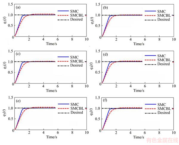
Figure 19 Comparison of experimental step response of SMC and SMCBL at joints 1 to 6 of IRB-120 robot

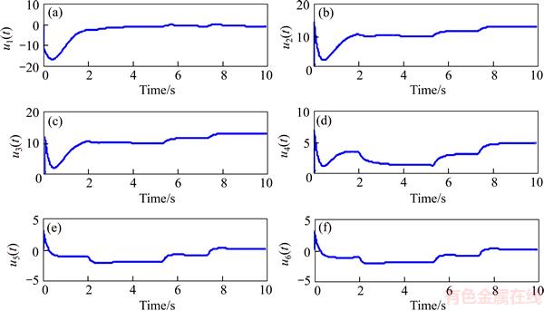
Figure 20 Experimental control input torques of SMCBL at joints 1 to 6 of IRB-120 robot

The proposed SMCBL controller is advantageous over SMC and IDC nonlinear controllers in terms of the transient state response, tracking error, and elimination of input signal chattering. It is a sufficient controller for an IRB-120 robot manipulator.

Notations

a_i

Link length

c_i

Cosine function of cosθ_i

c_ijk

Christoffel symbols

Matrix related to Coriolis and centrifugal terms

C_kj

Elements ofmatrix

d

External disturbance torque of system

d_i

Link offset

d_ij

Elements of D(q) matrix

D(q)

Inertia matrix

e

Exponential function of exp

e_ss

Steady-state error

e(t)

Position tracking error

Velocity tracking error

Acceleration tracking error

g₀

Gravitational constant

g_k(q)

Gravity elements

G(q)

Matrix related to gravity term

h_ci(q)

Height of ith link center of mass

H_∞

H-infinity

I_i

Inertia tensor matrix in the center of mass of ith link

J

Jacobian matrix of the robot

J_vi

Up half of Jacobean matrix

J_ωi

Down half of Jacobean matrix

K_i

Control parameter (a constant and positive value)

K

A gain control matrix and diagonal with positive elements of k_i

K_D

Derivative coefficient

K_I

Integral coefficient

K_P

Proportional coefficient

l_i

Distance between previous joint and center of mass of ith link

m_i

Mass of ith link of robot

M

Overshoot average

n

Number of system’s degrees of freedom

q_i

Position or angle of ith joint of the robot

q

Position of the robot’s joints

Velocity of the robot’s joints

Acceleration of the robot's joints

q(t)

Output of system (position of the robot)

q_d(t)

Desired output of system

Position tracking error

Velocity tracking error

R_i

Rotation homogeneous

transformations matrix of ith link

S_i

Sinusoidal function of sinθ_i

S(t)

Sliding surface

Derived sliding surface

Sat(S/φ)

Saturation function

Sign(S)

Sign function

t_r

Rise time

t_s

Setting time

T_s

Sampling time

Transformation matrix

u(t)

Control input torque (control input signal)

u

Total control input (the same control input τ(t))

Equivalent control input

α_i

Link twist

z

A positive constant

β

Setting parameter

η

A positive constant

θ_i

Joint angle

λ_i

Control parameter (a constant and positive value)

Λ

A diagonal eigenvalues matrix with elements of λ_i

v_e

Vector including linear velocity and angular velocity of end- effector

τ(t)

Control input torque related to robot joint torques

φ

Boundary layer thickness

Subscripts

ci

Center of mass of ith link

d

Desired

D

Derivative

I

Integral

P

Proportional

i

ith link of robot or ith joint of robot (i=1, …, 6)

ijk

Equal numbers 1, 2 and 3

v_i

Linear velocity of the center of mass of ith link

ω_i

Angular velocity of the center of mass of ith link

Abbreviations

D-H

Denavit-hartenberg

DOF

Degrees of freedom

DSP

Digital signal processor

GA

Genetic algorithm

IDC

Inverse dynamics controller

NP-hard

Nondeterministic polynomial-time hard

PID

Proportional-integral-derivative

SMC

Sliding mode control

SMCBL

Sliding mode control with boundary layer

Appendix: Calculation of optimal control parameters in Eq.(44)

In design and coding optimization algorithms such as genetic algorithms (GA), it is important to properly define the relevant cost functions. There is no general law by which to define a unique cost function for a problem, only a general procedure; thus, designers may define different cost functions for the same problem. The definition of a cost function should be carefully considered to find a fit cost function for a problem.

It is best to use specifications that affect the solutions of the considered problem in the criteria of the selected cost function. For an optimization problem, the aim is to optimize one or several parameters (such as λ_i and k_i control parameters) to find the best possible solutions for the parameters. To find the optimal solutions to the considered problem, it is first necessary to generate a number of solutions using an optimization algorithm. Following the generation of such solutions, the cost function is used to discover which solutions optimize the cost function, and these are considered as the final optimal solutions to the problem.

To calculate the optimal control parameters of λ_i and k_i in Eq. (44), first, a number of parameters were generated by the GA, and then the parameters were replaced in the cost function of Eq. (43). Control parameters λ_i and k_i that minimized the cost function of Eq. (43) were considered as optimal control parameters.

According to Eqs. (29) and (36), any change in λ_i and k_i will affect S and In addition, the solutions of the differential equation are shown in Eq. (29), where the primary condition becomesand when S=0 and respectively.

The first solution is for the steady-state response of the system in the sliding phase, and the second solution is for the transient state response of the system in the closing phase. In fact, these solutions are the step response and tracking error signals presented in Figures 15 and 16. If the cost function is considered as the sum of the two solutions in the form of Eq. (46), any change in the control parameter of λ_i indirectly changes the value of cost function f (according to and Eq. (46)).

           (47)

In Eq. (47), if and λt=β, Eq. (43) will be the result. Moreover, in Eq. (36), This implies that there is a linear relationship between S and This means that any change in the control parameter of k_i will change the value of and thus the value of S. Ultimately, any change in k_i can indirectly change the value of cost function f.

Note: To implement the GA in MATLAB, the “ga” command in the Optimization Toolbox was used. Please refer to the MATLAB help section for more information about this tool. It provides an example for finding the optimal value of several parameters at once.

References

[1] EDWARS M. Robots in industry: An overview [J]. Applied Ergonomics, 1984, 15(1): 45–53.

[2] SAGE H G, De MATHELIN M F, OSTERTAG E. Robust control of robot manipulators: A survey [J]. International Journal of Control, 1999, 72(16): 1498–1522.

[3] KOLHE J P, SHAHEED M, CHANDAR T S, TALOLE S E. Robust control of robot manipulators based on uncertainty and disturbance estimation [J]. International Journal of Robust and Nonlinear Control, 2013, 23(1): 104–122.

[4] KHOUKHI A, HAMAM Y. Optimal control for robot manipulators. in optimization, optimal control and partial differential equations [M]. Basel: Springer, 1992: 207–218.

[5] SADATI N, BABAZADEH A. Optimal control of robot manipulators with a new two-level gradient-based approach [J]. Electrical Engineering, 2006, 88(5): 383–393.

[6] HUANG A C, CHIEN M C. Adaptive control of robot manipulators: A unified regressor-free approach [M]. World Scientific, 2010.

[7] HSU S H, FU L C. A fully adaptive decentralized control of robot manipulators [J]. Automatica, 2006, 42(10): 1761–1767.

[8] CERVANTES I, ALVAREZ-RAMIREZ J. On the PID tracking control of robot manipulators [J]. Systems & Control Letters, 2001, 42(1): 37–46.

[9] JAFAROV E M,  M A, ISTEFANOPULOS Y. A new variable structure PID-controller design for robot manipulators [J]. IEEE Transactions on Control Systems Technology, 2005, 13(1): 122–130.

[10] PILTAN F, YARMAHMOUDI M H, SHAMSODINI M, MAZLOMIAN E, HOSAINPOUR A. PUMA-560 robot manipulator position computed torque control methods using Matlab/Simulink and their integration into graduate nonlinear control and Matlab courses [J]. International Journal of Robotics and Automation, 2012, 3(3): 167–191.

[11] BABAIASL M, GHANBARI A, NOORANI S. Anthropomorphic mechanical design and Lyapunov-based control of a new shoulder rehabilitation system [J]. Engineering Solid Mechanics, 2014, 2(3): 151–162.

[12] MAHMOOD M, MHASKAR P. Lyapunov-based model predictive control of stochastic nonlinear systems [J]. Automatica, 2012, 48(9): 2271–2276.

[13] WEN J T, MURPHY S H. PID control for robot manipulators [M]. Rensselaer Polytechnic Institute, 1990.

[14] KHELFI M, ABDESSAMEUD A. Robust H-infinity trajectory tracking controller for a 6 Dof PUMA 560 robot manipulator [C]// International Electric Machines & Drives Conference (IEMDC 2007). IEEE, 2007: 88–94.

[15] ANKELHED D. On design of low order H-infinity control [D]. Sweden: Linkping University Electronic Press, 2011.

[16] FAUSETT L. Fundamentals of neural networks: Architectures, algorithms, and applications [M]. USA: Prentice-Hall Press, 1994.

[17] KUMAR N, PANWAR V, SUKAVANAM N, SHARMA S P, BORM J H. Neural network based hybrid force/position control for robot manipulators [J]. International Journal of Precision Engineering and Manufacturing, 2011, 12(3): 419–426.

[18] KUMAR N, PANWAR V, SUKAVANAM N, SHARMA S P, BORM J H. Neural network-based nonlinear tracking control of kinematically redundant robot manipulators [J]. Mathematical and Computer Modelling, 2011, 53(9): 1889–1901.

[19] WANG L, CHAI T, YANG C. Neural-network-based contouring control for robotic manipulators in operational space [J]. IEEE Transactions on Control Systems Technology, 2012, 20(4): 1073–1080.

[20] YU L, FEI S, HUANG J, GAO Y. Trajectory switching control of robotic manipulators based on RBF neural networks [J]. Circuits, Systems, and Signal Processing, 2014, 33(4): 1119–1133.

[21] WANG L X. A course in fuzzy systems [M]. USA: Prentice-Hall Press, 1999.

[22] SONG Z, YI J, ZHAO D, LI X. A computed torque controller for uncertain robotic manipulator systems: Fuzzy approach [J]. Fuzzy Sets and Systems, 2005, 154(2): 208–226.

[23] PILTAN F, HAGHIGHI S T, SULAIMAN N, NAZARI I, SIAMAK S. Artificial control of PUMA robot manipulator: A review of fuzzy inference engine and application to classical controller [J]. International Journal of Robotics and Automation, 2011, 2(5): 401–425.

[24] SICILIANO B, SCIAVICCO L, VILLANI L, ORIOLO G. Robotics: Modelling, planning and control [M]// Advanced Textbooks in Control and Signal Processing. Springer, 2009: 29.

[25] SPONG M W, HUTCHINSON S, VIDYASAGAR M. Robot dynamics and control [M]. New York: John Wiley & Sons, 2004.

[26] BABAIASL M, GHANBARI A, NOORANI S M R. Mechanical design, simulation and nonlinear control of a new exoskeleton robot for use in upper-limb rehabilitation after stroke [C]// Biomedical Engineering (ICBME 2013). Iran: IEEE, 2013: 5–10.

[27] GHOBAKHLOO A, EGHTESAD M, AZADI M. Position control of a Stewart-Gough platform using inverse dynamics method with full dynamics [C]// International Workshop on Advanced Motion Control. IEEE, 2006: 50–55.

[28] SLOTINE J J E, LI W. Applied nonlinear control [M]. Englewood Cliffs, NJ: Prentice-Hall Press, 1991.

[29] PILTAN F, EMAMZADEH S, HIVAND Z, SHAHRIYARI F, MIRAZAEI M. PUMA-560 robot manipulator position sliding mode control methods using MATLAB/SIMULINK and their integration into graduate/undergraduate nonlinear control, robotics and MATLAB courses [J]. International Journal of Robotics and Automation, 2012, 3(3): 106–150.

[30] CORRADINI M L, FOSSI V, GIANTOMASSI A, IPPOLITI G, LONGHI S, ORLANDO G. Discrete time sliding mode control of robotic manipulators: Development and experimental validation [J]. Control Engineering Practice, 2012, 20(8): 816–822.

[31] CORRADINI M L, FOSSI V, GIANTOMASSI A, IPPOLITI G, LONGHI S, ORLANDO G. Minimal resource allocating networks for discrete time sliding mode control of robotic manipulators [J]. IEEE Transactions on Industrial Informatics, 2012, 8(4): 733–745.

[32] CAPISANI L M, FERRARA A, MAGNANI L. Second order sliding mode motion control of rigid robot manipulators [C]// Decision and Control. IEEE, 2007: 3691–3696.

[33] CAPISANI L M, FERRARA A, MAGNANI L. Design and experimental validation of a second-order sliding-mode motion controller for robot manipulators [J]. International Journal of Control, 2009, 82(2): 365–377.

[34] CAPISANI L M, FERRARA A. Trajectory planning and second-order sliding mode motion/interaction control for robot manipulators in unknown environments [J]. IEEE Transactions on Industrial Electronics, 2012, 59(8): 3189–3198.

[35] JIN M, LEE J, CHANG P H, CHOI C. Practical nonsingular terminal sliding-mode control of robot manipulators for high-accuracy tracking control [J]. IEEE Transactions on Industrial Electronics, 2009, 56(9): 3593–3601.

[36] BABAIASL M, GOLDAR S N, BARHAGHTALAB M H, MEIGOLI V. Sliding mode control of an exoskeleton robot for use in upper-limb rehabilitation [C]// Robotics and Mechatronics (ICROM 2015). Tehran, Iran: IEEE, 2015: 694–701.

[37] NEKOUKAR V, ERFANIAN A. Adaptive fuzzy terminal sliding mode control for a class of MIMO uncertain nonlinear systems [J]. Fuzzy Sets and Systems, 2011, 179(1): 34–49.

[38] PILTAN F, SULAIMAN N, ROOSTA S, GAVAHIAN A, SOLTANI S. Artificial chattering free on-line fuzzy sliding mode algorithm for uncertain system: Applied in robot manipulator [J]. International Journal of Engineering, 2011, 5(5): 360–379.

[39] PILTAN F, SULAIMAN N, ZARE A, ALLAHHDADI S, DIALAME M. Design adaptive fuzzy inference sliding mode algorithm: Applied to robot arm [J]. International Journal of Robotics and Automation, 2011, 2(5): 283–297.

[40] PILTAN F, AGHAYARI F, RASHIDIAN M R, SHAMSODINI M. A new estimate sliding mode fuzzy controller for robotic manipulator [J]. International Journal of Robotics and Automation, 2012, 3(1): 45–58.

[41] JALALI A, PILTAN F, GAVAHIAN A, JALALI M. Model-free adaptive fuzzy sliding mode controller optimized by particle swarm for robot manipulator [J]. International Journal of Information Engineering and Electronic Business, 2013, 5(1): 68.

[42] PILTAN F, NABAEE A, EBRAHIMI M, BAZREGAR M. Design robust fuzzy sliding mode control technique for robot manipulator systems with modeling uncertainties [J]. International Journal of Information Technology and Computer Science, 2013, 5(8): 123–135.

[43] SOLTANPOUR M R, KHOOBAN M H, SOLTANI M. Robust fuzzy sliding mode control for tracking the robot manipulator in joint space and in presence of uncertainties [J]. Robotica, 2014, 32(3): 433–446.

[44] SOLTANPOUR M R, OTADOLAJAM P, KHOOBAN M H. Robust control strategy for electrically driven robot manipulators: Adaptive fuzzy sliding mode [J]. IET Science, Measurement & Technology, 2014, 9(3): 322–334.

[45] SOLTANPOUR M R, KHOOBAN M H. A particle swarm optimization approach for fuzzy sliding mode control for tracking the robot manipulator [J]. Nonlinear Dynamics, 2013, 74(1, 2): 467–478.

[46] VEYSI M, SOLTANPOUR M R, KHOOBAN M H. A novel self-adaptive modified bat fuzzy sliding mode control of robot manipulator in presence of uncertainties in task space [J]. Robotica, 2015, 33(10): 2045–2064.

[47] WAI R J, YANG Z W. Adaptive fuzzy neural network control design via a T–S fuzzy model for a robot manipulator including actuator dynamics [J]. IEEE Transactions on Systems, Man, and Cybernetics: Part B (Cybernetics), 2008, 38(5): 1326–1346.

[48] WAI R J, HUANG Y C, YANG Z W, SHIH C Y. Adaptive fuzzy-neural-network velocity sensorless control for robot manipulator position tracking [J]. IET Control Theory & Applications, 2010, 4(6): 1079–1093.

[49] BACHIR O, ZOUBIR A F. Adaptive neuro-fuzzy inference system based control of puma 600 robot manipulator [J]. International Journal of Electrical and Computer Engineering, 2012, 2(1): 90–97.

[50] CHAUDHARY H, PANWAR V, PRASAD R, SUKAVANAM N. Adaptive neuro fuzzy based hybrid force/position control for an industrial robot manipulator [J]. Journal of Intelligent Manufacturing, 2016, 27(6): 1299– 1308.

[51] WANG L, CHAI T, ZHAI L. Neural-network-based terminal sliding-mode control of robotic manipulators including actuator dynamics [J]. IEEE Transactions on Industrial Electronics, 2009, 56(9): 3296–3304.

[52] SUN T, PEI H, PAN Y, ZHOU H, ZHANG C. Neural network-based sliding mode adaptive control for robot manipulators [J]. Neurocomputing, 2011, 74(14): 2377–2384.

[53] WAI R J, MUTHUSAMY R. Fuzzy-neural-network inherited sliding-mode control for robot manipulator including actuator dynamics [J]. IEEE Transactions on Neural Networks and Learning Systems, 2013, 24(2): 274–287.

[54] WAI R J, MUTHUSAMY R. Fuzzy-neural-network control for robot manipulator via sliding-mode design [C]// Control Conference (ASCC 2013). Asian: IEEE, 2013: 1–6.

[55] HU H, WOO P Y. Fuzzy supervisory sliding-mode and neural-network control for robotic manipulators [J]. IEEE Transactions on Industrial Electronics, 2006, 53(3): 929–940.

[56] KHOOBAN M H, NIKNAM T, BLAABJERG F, Dehghani M. Free chattering hybrid sliding mode control for a class of non-linear systems: Electric vehicles as a case study [J]. IET Science, Measurement & Technology, 2016, 10(7): 776–785.

[57] BARHAGHTALAB M H, MEIGOLI V. Robot manipulator position control using hybrid control method based on sliding mode and ANFIS with fuzzy supervisor [J]. International Journal of Control Theory and Applications, 2015, 8(4): 1281–1291.

[58] CRAIG J J. Introduction to robotics: mechanics and control [M]. Upper Saddle River: Pearson Prentice Hall, 2005.

(Edited by FANG Jing-hua)

中文导读

六自由度IRB-120机器人机械手的滑模控制与边界层控制

摘要：由于线性PID控制器易于实现，一般采用其对机器人进行控制。线性控制器不能有效地处理不确定性和参数的变化，因此推荐具有鲁棒性能的非线性控制器。滑模控制(SMC)是一种针对非线性系统的鲁棒状态反馈控制方法，其设计简单，有效地克服了系统中的不确定性和扰动，它的瞬态响应非常快，是理想的控制器。SMC最主要的缺点是控制输入信号的抖动。为了解决这一问题，本文采用SMC与边界层(SMCBL)相结合的方法，消除了系统的抖振现象，提高了系统的性能。将所提出的SMCBL与传统的非线性控制方法逆动态控制(IDC)进行了比较。首先，对IRB-120机器人机械手的运动学方程和动力学方程进行了完整、准确的提取；然后，对采用SMC的机器人机械手的控制进行了评价。为了验证该控制方法的有效性，在一个6自由度IRB-120机器人机械手上使用了该控制方法。在MATLAB/Simulink环境下对仿真结果进行了仿真、测试和比较。为了进一步验证我们的工作，在一个实际的IRB-120机器人机械手上进行了测试和实验验证。

关键词：机器人机械手控制；IRB-120机器人；滑模控制；带边界层的滑模控制；逆动态控制

Received date: 2017-06-26; Accepted date: 2017-11-28

Corresponding author: Mojtaba HADI BARHAGHTALAB, PhD Candidate; Tel: +98–71–36260232; E-mail: mh.barhaghtalab@ gmail.com; ORCID: 0000-0002-2571-3723