J. Cent. South Univ. (2016) 23: 2305-2313

DOI: 10.1007/s11771-016-3288-5

Forward modeling for “earth-ionosphere” mode electromagnetic field

LI Di-quan(李帝铨)^{1, 2}, XIE Wei(谢维)^{1, 2}, DI Qing-yun(底青云)³, WANG Miao-yue(王妙月)³

1. Key Laboratory of Metallogenic Prediction of Nonferrous Metals of Ministry of Education(Central South University), Changsha 410083, China;

2. School of Geosciences and Info-Physics, Central South University, Changsha 410083, China;

3. Institute of Geology and Geophysics, Chinese Academy of Sciences, Beijing 100029, China

Central South University Press and Springer-Verlag Berlin Heidelberg 2016

Abstract: A fixed artificial source (greater than 200 kW) was used and the source location was selected at a high resistivity region to ensure high emission efficiency. Some publications used the “earth-ionosphere" mode in modeling the electromagnetic (EM) fields with the offset up to a thousand kilometer, and such EM fields still have a signal/noise ratio of 10-20 dB. This means that a new EM method with fixed source is feasible, but in their calculation, the displacement in air was neglected. In this work, some three-layer modeling results were presented to illustrate the basic EM fields’ characteristics in the near, far and waveguide areas under “earth-ionosphere” mode, and a standard is given to distinguish the boundary of near, far and waveguide areas. Due to the influence of the ionosphere and displacement current in the air, the “earth-ionosphere” mode EM fields have an extra waveguide zone, where the fields’ behavior is very different from that of the far field zone.

Key words: earth-ionosphere mode; large power; large offset; electromagnetic field; forward modeling

1 Introduction

In communication area, extremely low frequency (ELF), electromagnetic waves 3 Hz-3 kHz were generally used for long-range communication and navigation with submarines due to their comparatively large skin depths in salt water and low attenuation. This technology can also be utilized in military communication [1-4]. The study on the propagation of such low-frequency radio waves was matured in communication area [5-10]. At the same time in the electromagnetic exploration area, the study on the propagation of 0.01 Hz-10 kHz electromagnetic (EM) wave was matured too [11]. In the former, the upper space above earth surface is mainly considered, while in the latter it is the lower space beneath earth surface that is mainly considered. In recent years, the study on the propagation of 0.1 Hz-300 Hz EM wave in complete whole space including ionosphere, air and earth has been proposed in geophysical prospection and earthquake prediction [12-15].

In magnetotellurics (MT), by measuring the natural variations of electrical and magnetic fields at the earth’s surface, the subsurface can be imaged. Due to the nature of MT source, long recording time is needed to ascertain usable readings due to the fluctuations and the low signal strength. In order to solve this problem, controlled source audio-frequency magnetotellurics (CSAMT) method has been developed by using a transmitter instead of relying on natural forces.The key advantage for the CSAMT method is that signals are stronger than MT and thus are more coherent. Data acquisition for the CSAMT method is much faster than MT surveys, so the overall survey costs can be reduced significantly. The key disadvantage for the CSAMT method relates to the “near field”effect which could distort the data.To overcome this problem, it was hoped that much greater offset can be applied. However, the offset of CSAMT cannot be greater than 20 km because of low emission energy (less than 30 kW).

A new artificial source EM sounding technique was thus proposed, in which a fixed high-power transmitting station is used (greater than 200 kW). The station is located at a high resistivity region (to ensure high emission efficiency), and the length of the source is up to tens of km; As an artificial signal source, stable SLE/ELF EM signal can then be created for exploration and earthquake prediction [12, 15]. As long as the source strength is strong enough, the artificial EM signal can be easily observed within several thousand kilometers [16-20]. Vast theoretical and experimental works with this new method have been done [12-15, 17-29]. There were some publications about 1D and 2D forward and inverse modeling [30-36]. In these publications, the main purpose is to get the answer whether the artificial EM signal can be achieved in the waveguide area, and some of them have obtained some results to help designing new instrument, especially giving some clues of the parameters of the EM emission system used in design.

The work develops a forward modeling method for geophysical exploration to estimate the signal magnitude. Such study is essential and most important in data processing and data interpretation. Earth-ionosphere mode model was constructed, in which the effect of ionosphere and displacement current in the air based on new mathematical derivation is included. In order to study the characteristics of EM fields in earth- ionosphere mode, the study on complex earth media for artificial source and large offset with R function method was conducted. Also, the EM fields decaying characteristics of given frequencies for the three-layer earth-ionosphere model was modeled, and the modeling results with the quasi static analytical results have been compared [11]. And the effect of ionosphere and displacement current in the air was analyzed and the boundary of near field, far field and waveguide field was provided.

2 Ionosphere model

The main purpose of this work is to calculate the electric and magnetic fields at some remote location at a horizontal distance r from the source. The earth- ionosphere waveguide is interpreted as a spherical cavity whose upper wall is horizontally characterized by inhomogeneous anisotropic impedance. By a simple approximation of the earth-ionosphere waveguide, which is nonetheless useful in many situations, the flat earth model is used. The waveguide is modeled as an infinite parallel plate waveguide with the curvature of the earth and the ionosphere neglected. This model is valid for the distances of up to half an earth radius from the source [8, 12, 37]. Assuming the impedance of earth-ionosphere waveguide to be small, its influence on the electromagnetic fields can be considered with an ideal cavity with infinitely upper walls [38], so flat earth- ionosphere model with infinitely upper walls in modeling was applied.

3 Earth-ionosphere mode EM model

Earth-ionosphere mode model was established. R function method that is similar to the CSAMT method was employed for the mathematical derivation, and the formulas of electric and magnetic fields component was deduced. The high sampling density Hankel digital filter method was used for numerical simulation [13]. In the communication area the earth-ionosphere mode is frequently earth spheres layered, whereas in the geophysical exploration area, the earth-ionosphere mode is horizontal plate layered of which the precision is high enough when the horizontal distance is significantly shorter than the radius of earth (i.e. 2500 km), and the exploration depth is less than 10 km [12]. Moreover, in geophysical exploration, the impendence is the very parameter that was considered most, and the impendence is the same for the spheres layered and horizontal plate layered, which was demonstrated to be true in MT.

The EM’s model in earth-ionosphere mode is schematically illustrated in Fig. 1. In the model, the layer index of ionosphere is -1; atmosphere is 0; earth is 1, …, n. The source (HED, with time factor e^-iωt) is put in the air and the distance between source and the surface of earth is h₀. Origin of the coordinate system was set in the center of the source, the downward of z-axis is positive, the upward is negative, and so the height of the ionosphere is negative. Assuming that both the thickness of ionosphere and the bottom stratum are infinite, the effective height of the bottom interface of ionosphere, the layer thickness of air, is 100 km. The effective resistivity of the ionosphere is taken as 10⁴ Ω·m. The relative dielectric constant ε and relative permeability μ are fixed to be 1.

Fig. 1 Schematic illustration of proposed earth-ionosphere mode

4 Theoretical derivations

With the vector potential A, the basic functions can be expressed as

                            (1)

where A is vector potential; Φ is scalar potential; E is electric vector; H is magnetic vector; μ is magnetic permeability; i is pure imaginary; ω is circular frequency; k is wave number; k²=-iωμ/ρ-ω²εμ; ε is permittivity; ρ is resistivity.

It was assumed that HED is along the x direction, the charge is accumulated nearby the interfaces of layers along the z direction, and there are vector potential along x (A_x) and z (A_z) direction.

The expressions of A_x, A_z and Φ are deduced after many steps with boundary conditions (2), which can be described as the Eqs. (3)-(5).

                     (2)

                       (3)

 (4)

   (5)

where A_p and A_p+1 are the vector potentials of p and p+1 layer, respectively; A_xp and A_xp+1 are the vector potentials of p and p+1 layer, respectively, along x direction; A_zp and A_zp+1 are the vector potentials of p and p+1 layers, respectively, along z direction. In this case,

where k_p is the wave number of p layer; λ is the spatial frequency; r is the offset; θ is the angle of r and x direction; P_E is the dipole moment; J₀(λr) and J₁(λr) are the Bessel function; R₁ and are the functions related to which contact with the earth layer resistivity and thickness, respectively. And the expressions of R₁ and are the same as CSAMT.

 (6)

                     (7)

All the electric fields components E_x, H_y and magnetic fields components H_x ,H_y, H_z can be derived from function (2). E_x and H_y frequently calculated by traditional CSAMT method are expressed as

              (8)

    (9)

The contributions of ionosphere and displacement current have been expressed in c_oc, c_od and respectively. The differences of c_oc, c_od and between traditional CSAMT model and earth- ionosphere model are the main causes of the differences of EM fields between the CSAMT model and the earth-ionosphere model. Whether the contribution of displacement current has been considered or not is depending on the selection of wave number k. If k²= -iωμ/ρ-ω²εμ, the contribution of displacement current is considered, if k²=-iωμ/ρ, the contribution of displacement current is neglected. Till now, the displacement current’s role on EM has been neglected, especially in the calculation of E_x and H_y in CSAMT. In this work, displacement current has been considered.

The solution of long line electric source can be obtained by numerical summation of the solutions obtained by Eqs. (8) and (9) of point sources along the long line.

5 Numerical simulations

In order to study the characteristics of three-layer media of the EM fields in earth-ionosphere mode, many cases of n were tested. Here only the results of the three- layer media of the earth-ionosphere mode EM fields are presented, which is enough to indicate the basic characteristics. The modeling of decay characteristics of electromagnetic fields was conducted, as shown in Fig. 2.

The coordination system is the same as that shown in Fig. 1. The layer indices of ionosphere, atmosphere, and earth is -1, 0, and 1, respectively. The resistivities of these three layers are of ρ_-1=10 kΩ·m, ρ₀=10¹¹ kΩ·m and ρ₁=5 kΩ·m, respectively. And the thicknesses of corresponding layers are h_-1=∞, h₀=100 km, and h₁=∞,respectively. The HED moment is 1×10⁷ A·m. The transmitted frequencies are 0.1, 5.0, and 300 Hz, respectively.

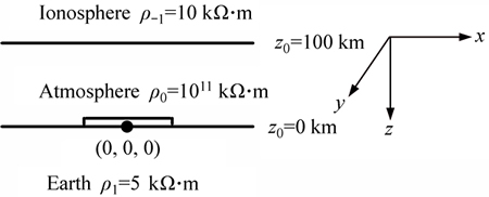
Fig. 2 Sketch including ionosphere whole space model

The receivers were placed on the earth surface with y=0 km, z=0 km and x=35-2500 km. The receivers for equatorial array are also on the earth surface: x=0 km, z=0 km and y has the same value as x for axial array.

Figures 3-5 show the decay curves of the earth- ionosphere mode fields’ of axial array for the frequency of 0.1 Hz, 5 Hz and 300 Hz, respectively. The solid lines are the earth-ionosphere mode modeling data taking into account of the displacement current. The dot lines are the earth-ionosphere mode modeling data without considering the displacement current. The dash lines are the quasi static field analytical results of the earth half space [1].

Figures 6-8 show the decay curves of equatorial array of the earth-ionosphere mode fields’ for the frequencies of 0.1 Hz, 5 Hz and 300 Hz, respectively.

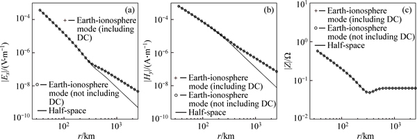
Fig. 3 |E_x| (a), |H_y| (b) and |Z| (c) fields decay curves for axial array (0.1 Hz)

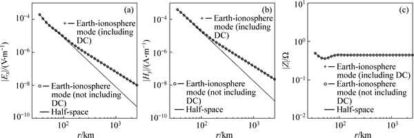
Fig. 4 |E_x| (a), |H_y| (b) and |Z| (c) fields decay curves for axial array (5 Hz)

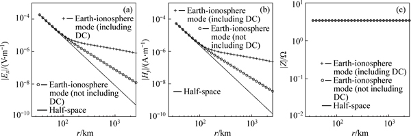
Fig. 5 |E_x| (a), |H_y| (b) and |Z| (c) fields decay curves for axial array (300 Hz)

Fig. 6 |E_x| (a), |H_y| (b) and |Z| (c) fields decay curves for equatorial array (0.1 Hz)

Fig. 7 |E_x| (a), |H_y| (b) and |Z| (c) fields decay curves for equatorial array (5 Hz)

Fig. 8 |E_x| (a), |H_y| (b) and |Z| (c) fields decay curves for equatorial array (300 Hz)

The decay lines shown in Figs. 3-8 indicate that no matter what frequencies were employed, both E_x and H_y fields of modeling (solid lines: considering the displacement current; dot lines: without considering the displacement current) and half space analytical (dash lines) for a small offset are identical because the ionosphere and displacement current effects are so small that it can be neglected. However, with the increase of offset, the effect of ionosphere becomes pronouncing and thus the differences between the E_x and H_y fields of modeling with or without considering the displacement current and analytical solution of half space model become very distinctive. The EM field amplitude of the earth-ionosphere mode is larger than that of the half space model, and the amplitude becomes even larger when including the displacement current. The difference appears at smaller offset with the frequency increasing. The difference for axial array is more obvious than equatorial array, which means that the polarization direction of EM fields is changing and the ellipse polarization phenomenon exits for large offset fields.

The right subplots of Figs. 3-8 indicate that impedances are identical, no matter what frequencies were employed, no matter considering displacement current or not, no matter considering the effect of ionosphere or not. That means that displacement current and ionosphere have effect on E_x and H_y, but have no effect on the impedance. At the large distances where displacement current and ionosphere are important for the EM fields, isn’t the impedance essentially. In far and waveguide fields, the induction response of impedance is the same as vertically incident plane wave.

Based on the numerical results of Figs. 3-8, the boundary determination of near field, far field and waveguide field for earth-ionosphere mode at different frequencies was achieved.

In earth-ionosphere mode, the EM waves’ behavior is the same as CSAMT (quasi-stable field) in near and far field. Because of small offset, the propagation of EM waves in the near and far field, mainly appeared as the distribution and induction of the conduction current, displacement current and effect of ionosphere can be neglected. The EM field is primarily a induced field (quasi-stable field). The propagation characteristics can be described by the theory of quasi-stable field which is analogous to classical theory of EM sounding. While in the waveguide field, EM waves run in a way completely different from near and far filed. The contribution of conduction current is so small in waveguide field that it can be neglected. Displacement current and ionosphere are taken into account, and the EM fields’ attenuation is much smaller than that in near and far field. In a word, the EM waves’ attenuation is large in the near and far fields, and becomes small in the waveguide field, which characterizes the varied spatial distributions and propagation of the induction and radiation fields [14].

It is an important but yet open issue how the “earth-ionosphere” mode EM waves distributed in the near, far and waveguide fields, how these zones link, and what their sizes are. There were two methods to distinguish far and waveguide fields. One is when the offset is greater than 3 times the height of ionosphere, the EM fields turn into waveguide field [3]. Another is when the EM fields of earth-ionosphere are larger than those of quasi-stable fields by 10%, the EM fields turn into waveguide field. The paper follows the division method proposed by Russian researches. Compartmentalizing boundary of near field and far field references to CSAMT. When the offset is greater than 3 times skin depth (when half length of the antenna is greater than 3 times skin depth, based on half length of the antenna), the EM fields turn into far field. The boundaries of near, far and waveguide field for earth- ionosphere mode at different frequencies are shown in Fig. 9.

The standard of boundary determination is not strict; the boundary between far and waveguide field is an area; there is no clear indication where the far field ends and waveguide field begins, just like that between near and far field, but the basic approximation features of EM fields in the near, far, waveguide area have already been seen. Under these standards, the boundaries of near and far fields at 0.1, 5 and 300 Hz are 338, 48 and 25 km, respectively. The boundary of waveguide field in axial direction is 350 km and the equatorial direction is 675 km at 0.1 Hz. When the frequency increses to 300 Hz, the axial direction is 110 km and the equatorial direction is 80 km.

Figures 10-13 show the E_x and H_y fields’ patterns of the earth-ionosphere mode and the modeling results are shown in Fig. 2. It can be seen that the attenuation of EM fields is the same at axial and equatorial directions at 0.1 and 5 Hz. But this phenomenon changes when frequency is 32 Hz at which the attenuation at axial direction is smaller than that of the equatorial direction. When the frequency further increases to 300 Hz, this phenomenon becomes even more evident. This is caused by the displacement current in the air.

Figures 10-13 can confirm that in earth-ionosphere mode there should be an extra waveguide zone for acting in a distance of several hundreds to thousands of kilometers, and there are many different characteristics between this extra zone and far field zone. The following difference can be observed: 1) the amplitudes of EM fields decay much slower; 2) the polarization patterns change; 3) the positions for better measurement of z_xy and z_yx changes; 4) there exits the polarization ellipse of electric and magnetic fields; 5) the long axis direction of the polarization ellipse in waveguide zone changes comparing to quasi static EM fields.

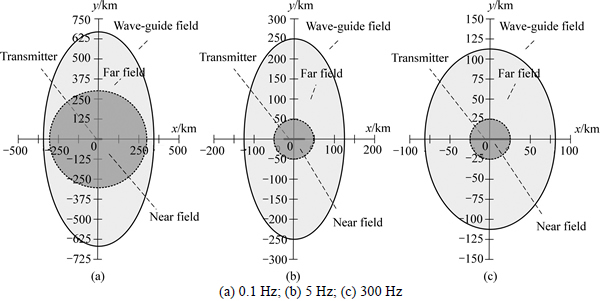
Fig. 9 Boundary of near, far and waveguide field:

Fig. 10 Radiation pattern of earth-ionosphere mode (0.1 Hz):

Fig. 11 Radiation pattern of earth-ionosphere mode (5 Hz):

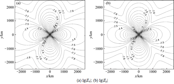
Fig. 12 Radiation pattern of earth-ionosphere mode (32 Hz):

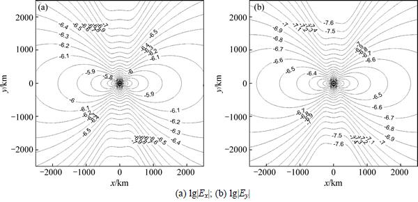
Fig. 13 Radiation pattern of earth-ionosphere mode (300 Hz):

6 Conclusions

1) Due to the influence of the ionosphere and displacement current in the air, the earth-ionosphere mode electromagnetic fields are very different from CSAMT. CSAMT fields only consider the near field zone and far field zone, but the earth-ionosphere mode EM fields have an extra waveguide zone where the fields’ behavior is very different from that of the far field zone.

2) Because the reflection effect of the ionosphere, the attenuation of electromagnetic wave in waveguide zone is small. Therefore, there exists a possibility that a fixed artificial source can be applied to excite the EM fields, in which not only strong enough magnitude, being used in geophysical exploration in near and far field within 20 km from source, is created, but also geophysical exploration in very far area reaching several thousand km from source so called waveguide area is feasible.

3) As a result of the effect of the displacement current in the air, the electromagnetic wave in the axial direction is greater than that of the equatorial direction, and as the frequency increases, the effect becomes more evident.

References

[1] WAIT J R. An extension to the mode theory of VLF ionospheric propagation [J]. Journal of Geophysical Research, 1958, 63(1): 125-135.

[2] WAIT J R. The long wavelength limit in scattering from a dielectric cylinder at oblique incidence [J]. Canadian Journal of Physics, 1965, 43(12): 2212-2215.

[3] BANNISTER P R, WILLIANMS F J. Results of the August 1972 Wisconsin test facility effective earth conductivity measurements [J]. Journal of Geophysical Research, 1974, 79(5): 725-732.

[4] CHANG D C, WAIT J R. Extremely low frequency (ELF) propagation along a horizontal wire located above or buried in the earth [J]. IEEE Transactions on Communications, 1974, 22(4): 421-427.

[5] GREIFINGER C, GREIFINGER P. Approximate method for determining ELF eigenvalues in the earth-ionosphere waveguide [J]. Radio Science, 1978, 13(5): 831-837.

[6] GREIFINGER C, GREIFINGER P. On the ionospheric parameters which govern high-latitude ELF propagation in the earth- ionosphere waveguide [J]. Radio Science, 1979, 14(5): 889-895.

[7] BANNISTER P R. ELF propagation update [J]. IEEE Journal of Oceanic Engineering, 1984, 9(3): 179-188.

[8] CUMMER S A. Modeling electromagnetic propagation in the earth-ionosphere waveguide [J]. IEEE Transactions on Antennas and Propagation, 2000, 48(9): 1420-1429.

[9] GALEJS J. Terrestrial propagation of long electromagnetic waves: International series of monographs in electromagnetic waves [M]. Oxford: Elsevier, 2013.

[10] WAIT J R. Electromagnetic waves in stratified media: Revised edition including supplemented material [M]. Oxford: Elsevier, 2013.

[11] WARD S H, HOHMANN G W. Electromagnetic theory for geophysical applications [J]. Electromagnetic Methods in Applied Geophysics, 1988, 1(3): 130-311.

[12] ZHUO Xian-jun, ZHAO Guo-zhe. A new technique of EM controlled-source sounding for resource prospecting [J]. Oil Geophysical Prospecting, 2004, 39(B11): 114-117. (in Chinese)

[13] LI Di-quan, DI Qing-yun, WANG Miao-yue. One-dimensional electromagnetic fields forward modeling for earth-ionosphere mode [J]. Chinese Journal of Geophysics, 2011, 54(9): 2375-2388. (in Chinese)

[14] YANG Jing. Propagation characteristics of CSELF electromagnetic waves [D]. Beijing: Institute of Geology, China Earthquake Administration, 2011. (in Chinese)

[15] ZHUO Xian-jun, LU Jian-xun, ZHAO Guo-zhe, DI Qing-yun. The extremely low frequency engineering project using WEM for underground exploration [J]. Engineering Science, 2011, 13(9): 42-50. (in Chinese)

[16] ZHUO Xian-jun. The research of the distribution and measurement of artificial SLF field [D]. Beijing: Institute of Geology, Chinese Earthquake Administration, 2005. (in Chinese)

[17] ZHUO Xian-jun, ZHAO Guo-zhe, DI Qing-yun, BI Wen-bin, TANG Ji, WANG Ruo. Preliminary application of WEM in geophysical exploration [J]. Progress in Geophysics, 2007, 22(6): 1921-1924. (in Chinese)

[18] DI Qing-yun, WANG Miao-yue, WANG Ruo, WANG Guang-jie. Study of the long bipole and large power electromagnetic field [J]. Chinese Journal of Geophysics, 2008, 51(6): 1917-1928. (in Chinese)

[19] ZHAO Guo-zhe, WANG Li-feng, TANG Ji, CHENG Xiao-bin, ZHAN Yan, XIAO Qi-bing, WANG Ji-jun, CAI Jun-tao, XU Guang-jing, WAN Zhan-sheng, WANG Xiao, YANG Jing, DONG Ze-ye, FAN Ye, ZHANG Ji-hong, GAO Yan. New experiments of CSELF electromagnetic method for earthquake monitoring [J]. Chinese Journal of Geophysics, 2010, 53(3): 479-486. (in Chinese)

[20] ZHUO Xian-jun, LU Jian-xun. Application and prospect of WEM to resource exploration and earthquake predication [J]. Ship Science and Technology, 2010, 32(6): 3-8. (in Chinese)

[21] FRASER S, ANTONY C, BERNARDI A, MCGILL P R, LADD M, HELLIWELL R A, VILLARD J O. Low-frequency magnetic field measurements near the epicenter of the Ms 7.1 Loma Prieta earthquake [J]. Geophysical Research Letters, 1990, 17(9): 1465-1468.

[22] SIMPSON J J, HEIKES R P, TAFLOVE A. FDTD modeling of a novel ELF radar for major oil deposits using a three-dimensional geodesic grid of the earth-ionosphere waveguide [J]. IEEE Transactions on Antennas and Propagation, 2006, 54(6): 1734-1741.

[23] SIMPSON J J, TAFLOVE A. Three-dimensional FDTD modeling of impulsive ELF propagation about the earth-sphere [J]. IEEE Transactions on Antennas and Propagation, 2004, 52(2): 443-451.

[24] YOSHIHIRO I, KAZUSHIGE O. Very low frequency earthquakes within accretionary prisms are very low stress-drop earthquakes [J]. Geophysical Research Letters, 2006, 33(9): 302-305.

[25] PALMER S J, RYCROFT M J, CERMACK M. Solar and geomagnetic activity, extremely low frequency magnetic and electric fields and human health at the earth’s surface [J]. Surveys in Geophysics, 2006, 27(5): 557-595.

[26] HARRISON R G, APLIN K L, RYCROFT M J. Atmospheric electricity coupling between earthquake regions and the ionosphere [J]. Journal of Atmospheric and Solar-Terrestrial Physics, 2010, 72(5): 376-381.

[27] SARAEV A K, PERTEL M I, PARFENT'EV P A, PROKOF'EV V E, KHARLAMOV M M. Experimental study of the electromagnetic field from a VLF radio set for the purposes of monitoring seismic activity in the North caucasus [J]. Izvestiya Physics of the Solid Earth, 1999, 35(2): 101-108.

[28] ZHAO Guo-zhe, TANG Ji, DENG Qian-hui. Artificial SLF method and the experimental study for earthquake monitoring in Beijing area [J]. Earth Science Frontiers, 2003, 10(1): 248-257. (in Chinese)

[29] ZHAO Guo-zhe, LU Jian-xun. Monitoring and analysis of earthquake phenomena by artificial SLF waves [J]. Engineering Science, 2003, 5(10): 27-33. (in Chinese)

[30] BERENGER J P. An implicit FDTD scheme for the propagation of VLF–LF radio waves in the earth–ionosphere waveguide [J]. Comptes Rendus Physique, 2014, 15(5): 393-402.

[31] LI Guo-zhe, GU Tang-tian, LI Keng. SLF/ELF electromagnetic field of a horizontal dipole in the presence of an anisotropic earth- ionosphere cavity [J]. Applied Computational Electromagnetics Society Journal, 2014, 29(12): 1102-1111.

[32] NICKOLAENKO A P, HAYAKAWA M. Spectra and waveforms of ELF transients in the earth-ionosphere cavity with small losses [J]. Radio Science, 2014, 49(2): 118-130.

[33] SURKOV V, HAYAKAWA M. Earth-ionosphere cavity resonator, in ultra and extremely low frequency electromagnetic fields [M]. New York: Springer, 2014: 109-144.

[34] WANG Hai-bing. Two dimensional forward and inverse modeling of the very low frequency electromagnetic method [D]. Beijing: China University of Geosciences, 2014. (in Chinese)

[35] XU Zhi-hai. Two dimensional forward modeling of very low frequency electromagnetic method [D]. Beijing: China University of Geosciences, 2014. (in Chinese)

[36] LI Di-quan, DI Qing-yun, WANG Miao-yue, NOBES D. Earth-ionosphere mode controlled source electromagnetic method [J]. Geophysical Journal International, 2015, 202(3): 1848-1858.

[37] PORRAT D, FRASER S, ANTONY C. Propagation at extremely low frequencies [J]. Wiley Encyclopedia of Electrical and Electronics Engineering, 1999, 26(12): 101-120.

[38] KIRILLOV V V. Two-dimensional theory of elf electromagnetic wave propagation in the earth-ionosphere waveguide channel [J]. Radiophysics and Quantum Electronics, 1996, 39(9): 737-743.

(Edited by YANG Hua)

Foundation item: Projects(41204054, 41541036, 41604111) supported by the National Natural Science Foundation of China

Received date: 2016-04-08; Accepted date: 2016-07-15

Corresponding author: XIE Wei, PhD; Tel: +86-731-88877075; E-mail: xw76676372@126.com