New self-calibration approach to space robots based on hand-eye vision
来源期刊:中南大学学报(英文版)2011年第4期
论文作者:刘宇 刘宏 倪风雷 徐文福
文章页码:1087 - 1096
Key words:space robot; self-calibration; cost function; hand-eye vision; particle swarm optimization algorithm
Abstract:
To overcome the influence of on-orbit extreme temperature environment on the tool pose (position and orientation) accuracy of a space robot, a new self-calibration method based on a measurement camera (hand-eye vision) attached to its end-effector was presented. Using the relative pose errors between the two adjacent calibration positions of the space robot, the cost function of the calibration was built, which was different from the conventional calibration method. The particle swarm optimization algorithm (PSO) was used to optimize the function to realize the geometrical parameter identification of the space robot. The above calibration method was carried out through self-calibration simulation of a six-DOF space robot whose end-effector was equipped with hand-eye vision. The results showed that after calibration there was a significant improvement of tool pose accuracy in a set of independent reference positions, which verified the feasibility of the method. At the same time, because it was unnecessary for this method to know the transformation matrix from the robot base to the calibration plate, it reduced the complexity of calibration model and shortened the error propagation chain, which benefited to improve the calibration accuracy.
J. Cent. South Univ. Technol. (2011) 18: 1087-1096
DOI: 10.1007/s11771-011-0808-1![]()
LIU Yu(刘宇)1, LIU Hong(刘宏)1, NI Feng-lei(倪风雷)1, XU Wen-fu(徐文福)2
1. State Key Laboratory of Robotics and System, Harbin Institute of Technology, Harbin 150001, China;
2. Mechanical Engineering and Automation, Harbin Institute of Technology Shenzhen Graduate School,
Shenzhen 518057, China
? Central South University Press and Springer-Verlag Berlin Heidelberg 2011
Abstract: To overcome the influence of on-orbit extreme temperature environment on the tool pose (position and orientation) accuracy of a space robot, a new self-calibration method based on a measurement camera (hand-eye vision) attached to its end-effector was presented. Using the relative pose errors between the two adjacent calibration positions of the space robot, the cost function of the calibration was built, which was different from the conventional calibration method. The particle swarm optimization algorithm (PSO) was used to optimize the function to realize the geometrical parameter identification of the space robot. The above calibration method was carried out through self-calibration simulation of a six-DOF space robot whose end-effector was equipped with hand-eye vision. The results showed that after calibration there was a significant improvement of tool pose accuracy in a set of independent reference positions, which verified the feasibility of the method. At the same time, because it was unnecessary for this method to know the transformation matrix from the robot base to the calibration plate, it reduced the complexity of calibration model and shortened the error propagation chain, which benefited to improve the calibration accuracy.
Key words: space robot; self-calibration; cost function; hand-eye vision; particle swarm optimization algorithm
1 Introduction
At present, the on-orbit service is paid more attention to and plays a more important role in, for example, construction and maintenance of the space station, reclaim and release of the satellite, and replacement of orbital replacement unit (ORU). Usually, these tasks rely on the space robot, especially for the unmanned on-orbit service vehicle. A vital premise of satisfactory fulfillment of the above tasks is to require higher pose accuracy for the space robot. However, the kinematic parameters of the space robot vary with extreme spatial temperature environment, so after launch a well-calibrated space robot on ground must be recalibrated to adapt to the variation.
To date, the kinematic calibration has still been a key issue on the robot, since it relates to the complicated and precise manipulation of the robot. It is necessary to identify kinematic parameters of the robot model and then correct their kinematic errors, especially when it is not possible to use absolute end point measurements for position feedback. Kinematic calibration can be divided into two categories, namely geometric parameter calibration and non-geometric parameter calibration, and most researchers concentrate on the former. There are plenty of literatures to discuss it. BEYER and WULFSBURG [1] developed a ROSY calibration system with two CCD cameras and a reference sphere that enabled pose accuracy to be improved for conventional arms and parallel robots. SUN and HOLLERBACH [2] presented an active robot calibration algorithm based on the determinant-based updating observability index and demonstrated it with the calibration simulation of a six-DOF PUMA 560 robot. KANG et al [3] introduced a new metrology method based on the Product-of-Exponentials formula and the modified dyad kinematics to calibrate the modular robot, but there were no calibration results to be given. Using the circle point analysis technique, NEWMAN et al [4] performed the calibration of a Motoman P-8 robot, which required external hardware to determine the manipulator end point positions in Cartesian space.
On the other hand, research on non-geometric parameter calibration has also got great progress. JUDD and KNASINSKI [5] analyzed non-geometric errors (gear train errors, joint and link flexibility, etc) and proposed an error model that can be used for identification with a common least squares procedure. LIGHTCAP et al [6] applied a 30-parameter flexible geometric model to the Mitsubishi PA10-6CE robot, considering the flexibility in the harmonic transmission. DROUET et al [7] decomposed the measured end-point error into generalized geometric and elastic errors and realized compensation for dynamic elastic effects. With a camera attached to the end effector, RADKHAH et al [8] used an extended forward kinematic model incorporating both geometric and nongeometric parameters to identify the KUKA KR 125/2 robot kinematic parameters.
Unlike the ground, often on orbit no external measurement device can be used for the calibration of the space robot; however, usually it carries its own one fixed on its end effector, such as camera and laser range finder. With them, the space robot can carry out its self-calibration. The problem has been extensively studied. RUIZ et al [9] developed a self-calibration method of the space robot based on neural network. After extensive experimentation, the recalibration system was installed in the REIS robot included in the space station mock-up at Daimler-Benz Aerospace. LIANG et al [10] proposed an adaptive self-calibration approach of hand-eye system based on visual feedback, and discussed its implementation using square root Kalman filtering techniques. An experimental stereo-vision-based hand-eye system was used to verify the technology. Besides, ZHUANG and MENG [11] calibrated a camera-equipped manipulator using a scale with the factor method. GONG et al [12] used a hybrid non-contact optical sensor (a combination of vision sensor and structured light) attached to the end-effector to implement self-calibration of a six-DOF robot manufactured by Staubli Company based on distance measurement rather than absolute position measurement. The laser pointer could also be used for self-calibration of a robot through line-based approach [13-15].
In this work, with the D-H method, the relative pose error model was built. Kinematic parameter identification based on PSO was introduced. A calibration simulation of a Six-DOF space robot was provided.
2 Error model of space robot
2.1 Outline of robot calibration system
As shown in Fig.1, the space robot was fixed on the +z surface (pointing to the center of the earth) of the flying base, and a camera was fixed on the end-effector. The robot calibration plate was a symbol observed by the camera, and it had four same holes whose positions had been determined precisely. So, by observing them using hand-eye vision, the relative pose between the camera and calibration plate coordinate frame could be measured.
In this work, a new self-calibration method was
proposed. Namely, in this process of robot calibration, it was needless to know the transformation matrix 0Tc between the robot base coordinate frame Σ0 and calibration plate coordinate frame Σc, and the relative pose errors between the two adjacent calibration positions rather than the conventional ones with respect to Σ0 would be used to calibrate the space robot.
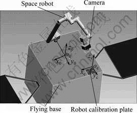
Fig.1 Sketch of space robot calibration system
As we knew, the temperature change on orbit was very violent, and it led to the fact that almost every dimension of the satellite would vary. In this case, it was also a very difficult thing to find a believable benchmark. So, to evade the transformation matrix, 0Tc in the calibration was an advantageous choice beyond doubt, and it was an important reason to utilize the relative pose to calibrate the space robot.
2.2 Kinematic model
Commonly, using the D-H parameter method, the relative translation and rotation from the robot link coordinate frame Σi-1 to Σi could be described by a homogeneous transformation matrix i-1Ai as
 (1)
(1)
where Cθi denotes cos(θi), Sθi denotes sin(θi), and the rest might be deduced by analogy. i-1Ai included four geometric parameters, namely θi, di, ai and αi. Among them, θi included two parts, i.e. initial joint angle θi0 and joint angle increment θi_inc.
It was well known that the method was inadequate when two successive rotational joints were parallel or nearly parallel. At that time, the common normal defining the distance between those two axes might be arbitrarily located, and if they were slightly nonparallel, this distance might greatly vary in magnitude. In the view of this, an extra parameter βi called the link twist angle around yi axis was introduced. By post-multipling the matrix i-1Ai by an additional rotation matrix R(yi, βi), the matrix i-1Ai could be changed as [16]

 (2)
(2)
where
 (3)
(3)
The twist angle βi was useful only for consecutive parallel or nearly parallel rotational joint axis. In this case, it was substituted for the joint offset di. For other cases, it was set as zero. According to the well-known loop closure equation, the homogeneous transformation 0Ti from Σ0 to the tool coordinate frame Σt could be given as
![]() (4)
(4)
where n denotes the number of the joint.
The space robot system could be simplified, as shown in Fig.2, where the real line denoted the configuration of the space robot in the first calibration position, and the dashed line represented the configuration in the second calibration position. Besides, it was assumed that ![]() represented the transformation matrix from base coordinate frame to the tool coordinate frame in the second calibration position. Obviously, the transformation matrix
represented the transformation matrix from base coordinate frame to the tool coordinate frame in the second calibration position. Obviously, the transformation matrix ![]() between the two tool coordinate frames in the two different calibration positions could be given as
between the two tool coordinate frames in the two different calibration positions could be given as
![]() (5)
(5)
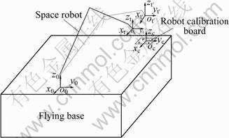
Fig.2 Relation between two adjacent calibration positions
As we knew, the transformation matrix tTc from Σt to Σc could be obtained by measurement of hand-eye vision. Likewise, ![]() could also be done. So, the following equation could be given:
could also be done. So, the following equation could be given:
![]() (6)
(6)
Attentively in the above formula, ![]() and tTc came from measurement, so
and tTc came from measurement, so ![]() was looked on as a measurement value. Comparatively
was looked on as a measurement value. Comparatively ![]() in Eq.(5) was a nominal value from the direct kinematic model whose geometric parameters would vary with outer environment. Easily, the matrix
in Eq.(5) was a nominal value from the direct kinematic model whose geometric parameters would vary with outer environment. Easily, the matrix ![]() could be divided into the following sub-matrix:
could be divided into the following sub-matrix:
![]() (7)
(7)
where ![]() denoted an orientation matrix; pn
denoted an orientation matrix; pn![]() R3, is a translational vector.
R3, is a translational vector.
2.3 Error model
As stated previously, these geometric parameters of the space robot would usually deviate from the nominal ones subjected to space environment. The geometric errors in the link i could be written as Δθi0, Δdi, Δai, Δαi and Δβi. Among them, Δθi0 denoted the initial joint angle error (also called as zero error), while the control error from joint angle increment θi_inc was not considered. Compared with their nominal parameter values, these errors could be looked on as a small deviation. If the real parameters of the link i were denoted by ![]() ,
, ![]() ,
, ![]() ,
, ![]() and
and ![]() , then the following formulas could be given:
, then the following formulas could be given:
 (8)
(8)
Generally ![]() was unequal to
was unequal to ![]() subjected to the above geometric parameter errors. If the geometric parameter errors higher than one-order error terms were omitted, according to differential transformation, the matrix
subjected to the above geometric parameter errors. If the geometric parameter errors higher than one-order error terms were omitted, according to differential transformation, the matrix ![]() could be written as
could be written as
![]() (9)
(9)
where ![]() was an orientation matrix; pc
was an orientation matrix; pc![]() R3, was a translational vector;
R3, was a translational vector; ![]() was an identity matrix;
was an identity matrix; ![]() was an operator that denoted a differential translational and rotational transformation matrix with respect to the coordinate system Σt.
was an operator that denoted a differential translational and rotational transformation matrix with respect to the coordinate system Σt.
Again, Δ could be written as
 (10)
(10)
where ![]() was a differential rotational matrix;
was a differential rotational matrix;
![]() was a one-order differential
was a one-order differential
translational vector.
Substituting Eqs.(7) and (10) into Eq.(9) yielded
![]() (11)
(11)
Further, the above formula could be simplified as
![]() (12)
(12)
where ![]() was a one-order position error vector with respect to the coordinate system Σt. δ=
was a one-order position error vector with respect to the coordinate system Σt. δ= ![]() was an one-order differential rotational vector, and it also denoted one-order orientation error.
was an one-order differential rotational vector, and it also denoted one-order orientation error.
3 Space robot calibration based on PSO
3.1 PSO algorithm
PSO, which resembled a school of flying birds, was originally developed by EBERHART and KENNEDY [17] to efficiently find the optimal or near-optimal solutions in large search spaces. In a particle swarm optimizer, instead of using genetic operators, these individuals were “evolved” by cooperation and competition among the individuals themselves through generations. Each individual, named as a “particle”, adjusted its flying according to its own flying experience and its flying experience of companions. It represented a potential solution to a problem, and was treated as a point in a D-dimensional space. The i-th particle was
![]() (13)
(13)
The best previous position (the position giving the best cost function value) of any particle was recorded and represented as
![]() (14)
(14)
And the best particle among all the particles in the population was denoted by
![]() (15)
(15)
The velocity of particle i was
![]() (16)
(16)
Then, the particles were manipulated according to the following formula:
![]() (17)
(17)
![]() (18)
(18)
where c1 and c2 were two positive constants, called the cognitive and social parameter respectively; rand( ) and Rand( ) were two random functions in the range [0,1]. The inertial weight w played the role of balancing the global search and local search. It could be a positive constant or even a positive linear or nonlinear function of time. The particle swarm optimizer had been found to be robust and fast in solving nonlinear, non-differentiable and multi-modal problems.
3.2 Cost function
The cost function was the object function optimized by PSO, and it determined optimization process and direction. Since PSO sought for a minimum function value, the cost function H for robot calibration could be chosen as
![]() (19)
(19)
where N denoted the number of calibration positions.
After the global search based on PSO was over, Pg could be given, namely, the geometric parameters deviating from the nominal ones were identified. However, Eq.(19) did not consider the difference of the units between the differential translational and rotational components. Simply, by weighing method, the above cost function was further expressed as
![]() (20)
(20)
where k was the adjusting factor that was used to balance the optimization of the position and orientation errors. If we were inclined to achieve higher position accuracy, the value k was increased; conversely, it was lessened.
3.3 Independent parameter
The initial joint configuration of the calibrated six-DOF space robot together with the coordinate system of each link was shown in Fig.3.
A complete calibration model consisted of a certain amount of independent geometric parameters. According to the formula developed by EVERETT et al [18], the six-joint space robot shown in Fig.3 had at most 30 identifiable independent parameters. However, the above calibration method only utilized the relative pose between the two adjacent calibration positions, and its independent geometric parameters would decrease. Eq.(5) could be extended into
![]() (21)
(21)
where

 (22)
(22)
Also
 (23)
(23)
Substituting Eqs.(22) and (23) into Eq.(21), θ10 could be cancelled. So, the first initial joint angle θ10 around the axis z0 made no difference to the relative poses. Further, θ10 could not be identified.
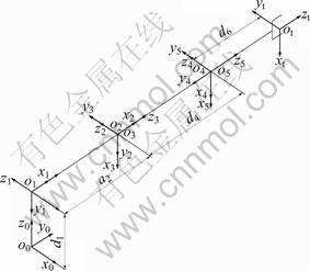
Fig.3 Link coordinate frames of six-DOF space robot
3.4 Calibration procedure based on PSO
One of the reasons that particle swarm optimization was attractive was that there were only very few parameters to adjust. Subsequently, PSO was used for the space robot calibration. Firstly, the i-th particle was defined as
![]()
![]() (24)
(24)
The population size was np, and the maximum number of iterations (epochs) to train was Nmax. The iterative ordinal number was denoted by k. Then, the summarized optimization procedure was as follows.
Step 1: Set k=1, and initialize a population of particles with random positions and velocities on D dimensions (here, D=23) in the solution space:
![]() (25)
(25)
Step 2: The cost function Hi of each particle was calculated by Eq.(20), namely
![]() (26)
(26)
Step 3: Calculate the previous best cost function Hi_best and the best position Pi for each particle:
 (27)
(27)
 (28)
(28)
Step 4: Calculate the best cost function Hg_best and the corresponding best particle Pg among all the particles in the population:
 (29)
(29)
 (30)
(30)
where Xi_min(k) is the best particle of i-th iteration.
Step 5: Change the velocity and position of the particle according to Eqs.(17) and (18), respectively.
Step 6: Loop to Step 2 until a criterion was met. Usually, a sufficiently good cost function value or a maximum number of iterations (Nmax) was obtained.
The velocities of the particles on each dimension were limited to a maximum velocity vmax. If the sum of accelerations caused the velocity on that dimension to exceed vmax specified by the user, then it was designated as vmax. Therefore, vmax was an important parameter, and it determined the resolution and which regions between the present position and the target (best so far) position were searched. If vmax was too high, particles might fly past good solutions. If it was too low, on the other hand, particles might not explore sufficiently beyond locally good regions. In fact, they could become trapped in local optima, unable to move far enough to reach a better position in the solution space.
4 Calibration simulation
4.1 Measurement noise
The previous Eq.(8) only considered the geometric parameter errors of the robot itself, but measurement noise caused by hand-eye vision was neglected. In fact, its measurement accuracy was often not high enough so as to influence the calibration effect of space robot. So, measurement noise had to be considered to improve the reality and availability of the simulation.
Here, we assumed that the random measurement noise vector ![]() followed a normal distribution with independent components and zero mean. If measurement accuracy was given as the maximum possible error (3σ), the measurement error specified in terms of the standard deviation was one third of the value. In that case, 99.7% of the error would be within the maximum error bound specified. In this work, the position and orientation measurement accuracies of hand-eye vision were given as 2.4 mm and 0.3°, respectively.
followed a normal distribution with independent components and zero mean. If measurement accuracy was given as the maximum possible error (3σ), the measurement error specified in terms of the standard deviation was one third of the value. In that case, 99.7% of the error would be within the maximum error bound specified. In this work, the position and orientation measurement accuracies of hand-eye vision were given as 2.4 mm and 0.3°, respectively.
In order to reduce the disturbance of stochastic measurement noise, in each calibration, position measurements would be repeated many times; then their mean was evaluated; at last it was added to the calibration model. Of course, it was not enough that measurement noise was filtered only by averaging. On the other hand, more redundant calibration positions were used to calibrate the space robot to further reduce the disturbance from measurement noise.
The transformation matrix could also be represented in the form of (px, py, pz, α, β, γ), where px, py and pz were the three components of the position vector and α, β and γ denoted the RPY angles. Because the measurement value equaled the sum of the real value and measurement noise, tTc and t′Tc could be simulated with the real geometric parameters and stochastic noise, which were used for the simulation.
4.2 Simulation of pose error
Since the space robot calibration was ready to be verified through simulation, the above pose measurement values were given by calculating. The detailed steps of generation of relative pose errors were listed as follows.
Step 1: Input all sets of chosen calibration positions, and the nominal and real geometric parameters of the space robot;
Step 2: Calculate the two transformation matrixes 0Tt and 0Tt′ with the nominal geometric parameters in the two adjacent calibration positions and then evaluate ![]() ;
;
Step 3: Calculate the two transformation matrixes ![]() and
and ![]() with the real geometric parameters in the two adjacent calibration positions and represent them as the pose vectors;
with the real geometric parameters in the two adjacent calibration positions and represent them as the pose vectors;
Step 4: Generate n stochastic measurement noise vectors repeatedly for each of the two adjacent calibration positions in terms of the above normal distribution and evaluate their mean;
Step 5: Add the two means to the above two real pose vectors and turn them into the transformation matrixes and so obtain tTc and t′Tc, at last evaluate![]() ;
;
Step 6: According to Eqs.(9) and (12), evaluate the position and orientation error vectors dp and δ.
4.3 Initial condition
The D-H parameters and their pre-assumed parameter errors of the space robot were listed in Table 1 and Table 2, respectively.
Here, considering the space robot working on orbit lighted by the sun, the above parameter errors ?ai and ?di were given a positive number. ?αi, ?βi and ?θi were given based on a normal distribution with zero mean and standard deviation of 0.2°.
Table 1 Nominal D-H parameters of space robot
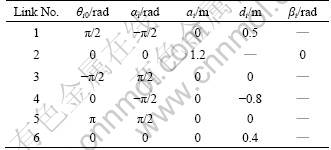
Table 2 Pre-assumed D-H parameter errors
The parameters of the particle swarm algorithm were assigned as Vmax=2.1, np=23, Nmax=500, c1=c2=2, and w=0.72.
4.4 Simulation result
Subsequently, the above calibration method of the space robot would be verified through simulation. Here, we had totally chosen 40 calibration positions where the joint configurations of the space robot were non-singular. Then, the two cases were simulated, namely 16 calibration positions and 10 repetitions, and 40 calibration positions and 10 repetitions. X repetition denoted the number of repeated measurements for a certain calibration position.
Besides, an independent set of reference positions (20 positions) distributed in the whole workspace of the space robot was selected to value the calibration effect.
Figure 4 showed the convergence process of the cost function optimized by the particle swarm algorithm. It was easy to see that the curve of the cost function declined steeply in the beginning, then turned gentle little by little, at last ended with the stopping criteria (500 iterations). The particle swarm algorithm behaved very stably under the condition of disturbance of larger measurement noise, which proved its strong stochastic adaptive search ability.
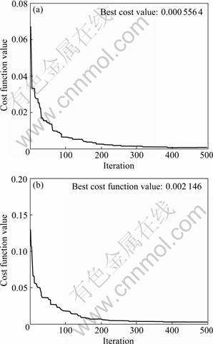
Fig.4 Variations of cost function values: (a) First case; (b) Second case
Figures 5(a) and (b) showed the position and orientation error curves calculated with the nominal geometric parameters in the calibration positions for the first case, respectively. Correspondingly, Figs.5(c) and (d) showed those calculated with the identified geometric parameters. Similarly, Figs.6(a), (b), (c) and (d) were for the second case.
Figures 7(a) and (b) showed the position and orientation error curves calculated with the nominal geometric parameters in the reference positions, respectively. Likewise, Figs.7(c) and (d) showed those calculated with the identified parameters for the first case, and Figs.7 (e) and (f) were for the second case.
According to Fig.5 and Fig.6, we could find that after parameter calibration, the pose accuracy of the space robot had a great improvement in the calibration position. However, in the reference position it would descend in a certain degree, especially for the first case, as shown in Fig.7. In nature, the robot calibration was fit for the measurement data in the calibration positions, and beyond them a discount of pose accuracy was inevitable. Moreover, in the reference position, the calibration effect for the second case was better than that for the first case, which meant that increasing the redundant calibration positions could enhance generalization and decrease the disadvantageous influence of measurement noise on the robot calibration.
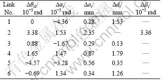
Tables 3 and 4 gave the identified geometric parameter errors for the first and second case, respectively. Table 5 gave a statistical comparison of the position and orientation errors calculated with the nominal parameters and identified ones in the reference positions. Here, the position and orientation errors all indicated the resultant errors of the three components of the position or orientation vectors, for instance, the resultant position error was represented as sqrt(x*x+y*y+ z*z). Attentively, in principle orientation, errors could not be synthesized because of mutual dependence of its three components, but here they were in a tiny magnitude and could be considered independent on each other. As shown in Table 5, for the first case, the maximum position and orientation errors respectively decreased from 17.599 mm and 10.377×10⁻³ rad to 5.548 mm and 3.309×10⁻³ rad; equivalently the calibration led to an improvement of pose accuracy by a factor of three or so. In contrast, for the second case these errors decreased to 2.744 m and 2.255×10⁻³ rad. The position accuracy was improved by up to 6.4 times and orientation accuracy by 4.6 times. Similarly, the comparison of the RMS (root mean square) pose errors could be given. Comparatively, the calibration results for the second case were better than those for the first case as a whole, which corresponded with the previous analysis. If more calibration positions were added, better results could be expected. Of course, as stated previously, using the calibration method, the geometric parameter θ10 could not be identified, and it would lead to an incomplete calibration model, which would influence the pose accuracy after calibration in a certain extent.

Fig.5 Pose errors calculated with nominal ((a) and (b)) and identified ((c) and (d)) parameters in calibration positions for first case: (a), (c) Position error; (b), (d) Orientation error
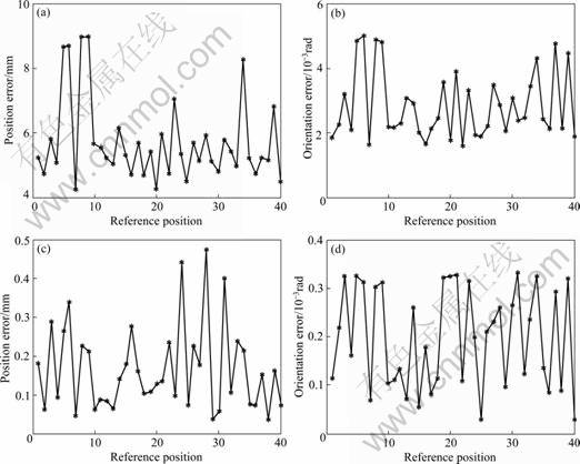
Fig.6 Pose errors calculated with nominal ((a) and (b)) and identified ((c) and (d)) parameters in calibration positions for second case: (a), (c) Position error; (b), (d) Orientation error
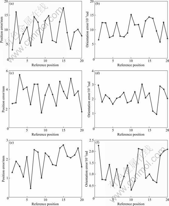
Fig.7 Pose errors calculated with nominal ((a) and (b)) and identified parameters ((c)-(f)) in reference positions: (a), (c) and (e) Position error; (b), (d) and (f) Orientation error; (c), (d) For first case; (e), (f) For second case
Table 3 Identified D-H parameter errors of space robot for first case
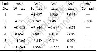
Table 4 Identified D-H parameter errors of space robot for second case
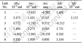
Table 5 Position and orientation error comparison after calibration

5 Conclusions
1) Using the relative pose errors between the two adjacent calibration positions, a self-calibration method of the space robot equipped with hand-eye vision was presented. It was unnecessary to know beforehand the transformation matrix between the robot base and the calibration plate, and benefited to simplify the calibration model and shorten the error propagation chain.
2) The number of the calibration positions had a great influence on the pose accuracy of space robot after calibration. More calibration positions could weaken the localization of chosen positions and bring better generalization. Besides, more calibration positions filtered measurement noise more effectively.
3) The particle swarm algorithm was fit for robot calibration, and it behaved very stably in the optimization process under the condition of disturbance of larger measurement noise. Attentively, the choice of velocities of the particles on each dimension should be adequate.
References
[1] BEYER L, WULFSBURG J. Practical robot calibration with rosy [J]. Robotica, 2004, 22(5): 505-512.
[2] SUN Y, HOLLERBACH J M. Active robot calibration algorithm [C]// Proceedings of ICRA 2008 IEEE International Conference on Robotics and Automation. Pasadena, 2008: 1276-1281.
[3] KANG S H, PRYOR M W, TESAR D. Kinematic model and metrology system for modular robot calibration [C]// Proceedings of ICRA 2004 IEEE International Conference on Robotics and Automation. Barcelona, 2004: 2894-2899.
[4] NEWMAN W S, BIRKHIMER C E, HORNING R J, WILKEY A T. Calibration of a Motoman P8 robot based on laser tracking [C]// Proceedings of the 2000 IEEE International Conference on Robotics and Automation. San Francisco, 2000: 3597-3602.
[5] JUDD R P, KNASINSKI A B. A technique to calibrate industrical robots with experimental verification [C]// Proceedings of IEEE Int Conf Robotics and Automation. Raleigh, 1987: 351-357.
[6] LIGHTCAP C, HAMMER S, SCHMITZ T, BANKS S. Improved positioning accuracy of the PA10-6CE robot with geometric and flexibility calibration [J]. IEEE Transactions on Robotics, 2008, 24(2): 452-456.
[7] DROUET P, DUBOWSKY S, ZEGHLOUL S, MAVROIDIS C. Compensation of geometric and elastic errors in large manipulators with an application to a high accuracy medical system [J]. Robotica, 2002, 20: 341-352.
[8] RADKHAH K, HEMKER T, STRYK O. A novel self-calibration method for industrial robots incorporating geometric and non-geometric Effects [C]// International Conference on Mechatronics and Automation. Takamatsu, 2008: 864-869.
[9] RUIZ V, ANGULO D, TORRAS C. Self-calibration of a space robot [J]. IEEE Trans on Neural Network, 1997, 8(4): 951-962.
[10] LIANG P, CHANG Y L, HACKWOOD S. Adaptive self-calibration of vision-based robot systems [J]. IEEE Transactions on Systems Man and Cybernetics, 1989, 19(4): 811-823.
[11] ZHUANG Han-qi, MENG Yan. Using a scale: Self-calibration of a robot system with factor method [C]// Proceedings of the 2001 IEEE Int. Conf. on Robotics and Automation. Seoul, 2001: 2797-2803.
[12] GONG Chun-he, YUAN Jing-xia, NI Jun. Nongeometric error identification and compensation for robotic system by inverse calibration [J]. International Journal of Machine Tools & Manufacture, 2000, 40(14): 2119-2137.
[13] LIU Y, SHEN Y T, XI X. Rapid Robot/Workcell Calibration Using Line-based Approach [C]// The 4th IEEE Conf on Automation Science and Engineering. Washington D C, 2008: 510-515.
[14] ZHUANG Han-qi, ROTH Z S, WANG K. Robot calibration by mobile camera system [J]. Robotic Systems, 1994, 11(3): 155-68.
[15] RENAUD P, ANDREFF N, MARQUET F, MARTINET P. Vision-based kinematic calibration of a H4 parallel mechanism [C]// Proceedings of IEEE Int Conf Robotics and Automation. Taipei, 2003: 1191-1196.
[16] VEITSCHEGGER W K, WU C H. Robot accuracy analysis based on kinematics [J]. IEEE Transactions on Robotics and Automation, 1986, 2: 171-180.
[17] EBERHART R C, KENNEDY J. A new optimizer using particle swarm theory [C]// Proceedings of the Sixth International Symposium on Micro Machine and Human Science. Nagoya, 1995: 39-43.
[18] EVERETT L, DRIELS M, MOORING B. Kinematic modeling for robot calibration [C]// Proceedings of IEEE Int Conf on Robotics and Automation. Raleigh, 1987: 183-190.
(Edited by YANG Bing)
Foundation item: Projects(60775049, 60805033) supported by the National Natural Science Foundation of China; Project(2007AA704317) supported by the National High Technology Research and Development Program of China
Received date: 2010-05-20; Accepted date: 2010-09-14
Corresponding author: LIU Yu, Associate Professor, PhD; Tel: +86-451-86402330; E-mail: lyu11@hit.edu.cn

