Trans. Nonferrous Met. Soc. China 28(2018) 1216-1225

Numerical simulation of friction stir butt-welding of 6061 aluminum alloy

Peng-cheng ZHAO, Yi-fu SHEN, Guo-qiang HUANG, Qi-xian ZHENG

College of Materials Science and Technology, Nanjing University of Aeronautics and Astronautics, Nanjing 210016, China

Received 24 February 2017; accepted 13 November 2017

Abstract: A two-dimensional computational fluid dynamics model was established to simulate the friction stir butt-welding of 6061 aluminum alloy. The dynamic mesh method was applied in this model to make the tool move forward and rotate in a manner similar to a real tool, and the calculated volumetric source of energy was loaded to establish a similar thermal environment to that used in the experiment. Besides, a small piece of zinc stock was embedded into the workpiece as a trace element. Temperature fields and vector plots were determined using a finite volume method, which was indirectly verified by traditional metallography. The simulation result indicated that the temperature distribution was asymmetric but had a similar tendency on the two sides of the welding line. The maximum temperature on the advancing side was approximately 10 K higher than that on the retreating side. Furthermore, the precise process of material flow behavior in combination with streamtraces was demonstrated by contour maps of the phases. Under the shearing force and forward extrusion pressure, material located in front of the tool tended to move along the tangent direction of the rotating tool. Notably, three whirlpools formed under a special pressure environment around the tool, resulting in a uniform composition distribution.

Key words: aluminum alloy; friction stir welding; numerical simulation; dynamic mesh; trace element method; temperature distribution; whirlpools

1 Introduction

Friction stir welding (FSW), an efficient solid-state joint process invented by the Welding Institute in 1991 [1], has been widely used in the full-scale production of certain products, such as rocket fuel tanks, operating mechanisms and ferry boats [2]. As a solid-state connection process, FSW has an enormous advantage over conventional fusion joining techniques, especially for dissimilar alloy connections. The knowledge of material flow behavior in FSW plays a fundamental role in determining the tool geometry and process parameters of the weld [3]. Tool angular velocity, welding velocity and plunge depth are basic parameters during the FSW process that have a substantial influence on the temperature distribution of the workpiece [4,5], the material flow behavior [6] and the mechanical and metallurgical characterization of the joint [7].

The progress in numerical temperature simulations of FSW has been achieved by researchers, and numerical analysis has found widespread application. KIRAL [8] obtained the temperature distribution in welding aluminum plates through transient thermal finite element analyses. A moving source with a thermal distribution simulating the heat generated by friction between the tool and the workpiece was used in a heat transfer analysis [9]. Contact conditions have a significant influence on the heat generation distribution, and the heat from the source is low when the rotational speed decreases. The moving source was shown to play an important role in this model. ZHANG et al [10] showed that the friction between the tool and workpiece was the main contributor to the temperature increase in the FSW process, but the contribution of plastic deformation increased as the welding speed increased. COX [11] studied the ability to control the temperature of the tool, which would provide more stability to the FSW process itself. NAIDU [12] found that the temperature difference along the z-direction was less than 10 K for the welding of Al7050 alloy, and the temperature distribution in different depths remained similar.

Many researchers have investigated the softened material flow behavior of the FSW process and achieved promising results. The marker insert technique (MIT) was applied to FSW to visualize the material transport using reconstruction of the piecewise cutoff welded zone. A good, qualitative characterization of the material flow behavior was achieved [13]. However, this study did not visualize the actual path of the material flow. ZHANG  et al [14] attempted to describe the path of the material flow in FSW using tracer elements combined with simulation; however, the description was not sufficiently clear to explain the material flow behavior because the tracer element was not shown in his model. Tracers were used in Pashazadeh’s research [15] to show the material flow behavior around the pin, which allowed a better understanding of the welding mechanism. A FSW numerical model for 2014 aluminum alloy was developed based on fluid mechanics, and visualization experiments of material flow behavior employing MIT were conducted to validate the simulation results [16]. The results showed that the material close to the welding line flowed vertically. On the advancing side, the material was pushed down, and on the retreating side, the material was pushed up. Similar results were shown in another study [17].

Although some numerical simulations have been performed to investigate the thermal and material flow behavior during FSW, there are limited researches focusing on the linear motion of the rotating tool. In this study, the coupled Eulerian/Langrangian computation method was employed. The workpiece was treated as an Eulerian component, while the rotating tool was treated as a Lagrangian component. The coupled Eulerian/ Lagrangian computational analysis of the FSW process had two-way thermo-mechanical characteristics. Temperature was allowed to affect the mechanical aspects of the model through temperature-dependent material properties. Combined with the dynamic mesh, the unsteady material flow process was displayed using the transient temperature distribution. Flow vectors and streamtraces were used to show the continuous process of material flow. The simulation results were validated by a visualization experiment from both aspects.

2 Experimental

Figure 1 depicts the schematic diagram of the FSW process and the observation and simulation plane. Two 6061 aluminum alloy plates (150 mm × 50 mm × 8 mm) were welded together using FSW technology. A small piece of zinc stock (20 mm × 3 mm × 4 mm) was embedded into the advancing side, which was used to track the flow behavior as marker material. The zinc stock was placed at the middle of the plate. The observation plane was perpendicular to the tool axis and was 3 mm away from the top surface, which was also the simulation plane of the following model. The tool rotated at a speed of 800 r/min and moved forward with a speed of 30 mm/min. The shoulder applied a pressure of 12 MPa to the workpiece. The FSW procedures were performed using a numerically controlled milling machine with a tool of H13 quenched and tempered  steel, which had a shoulder of 24 mm in diameter and a unthreaded conical pin of 6 mm in root diameter, 5 mm in tip diameter, and 6 mm in length.

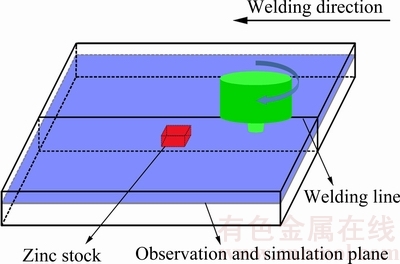
Fig. 1 Schematic diagram of FSW and simulation plane

Eight TP-02 surface-contact thermocouples were embedded into two plates symmetrically at the same height as that of the observation plane to measure the change in temperature at the eight different monitoring points. The thermocouples recorded different temperature-time (T-T) curves due to different thermal environments of every monitoring point. The T-T curves measured in the experiment were used to check the temperature distribution attained by numerical simulation and to verify the reasonability of the thermal environment.

3 Numerical modeling

A two-dimensional finite volume element (FVM) model of the FSW process, considering temperature, pressure, motion vector and strain, was established to study the thermal environment and the material flow behavior, which are usually obtained by setting the proper parameters in the standard computational fluid dynamics (CFD) software. Fluent, which is a common CFD tool to model the material flow behavior, was used to model the FSW process in this study.

3.1 Model description

To conduct the numerical simulation successfully, an important assumption must be made to simplify the real physical process: the material to be welded is treated as a non-Newtonian, incompressible, viscous-plastic material [15], indicating that material flow behavior will be easy only if the material viscosity is sufficiently low.

The FSW process contains a dynamic motion, therefore, it needs an unsteady implicit solver to solve the project, which is a pressure-based solver by default. Considering the two types of materials used during the welding, it is also essential to choose a reasonable multiphase model to define the two different phases. Compared with the volume of fluid model and the mixture model, the Eulerian model has several advantages in the simulation of FSW [18]. The Eulerian solves a set of momentum and continuity equations for each phase. Coupling is achieved through the pressure and inter-phase exchange coefficients. There is no difference between the liquid-liquid model and liquid-granular model, indicating that different softened phases in FSW can be solved well.

Figure 2 shows several mesh plots that reveal the re-meshing process during the simulation of the FSW. The whole region was divided into two pieces: the groove region, which included the base metal, and the flow-capable region in which the metal was softened and flowed during the welding, as shown in Fig. 2(a). The groove region where both the momentum and heat equations were solved was filled with rectangular cells because it did not suffer a distortion and remained rectangular. However, the flow-capable region where only the heat equation was solved must be filled with triangular cells because new triangular cells would be created with the distortion and disappearance of the original triangular cells in the re-meshing process.

The dynamic mesh model was used to model material flow where the shape of the domain changed with time due to the motion of domain boundaries. The tool’s movement in FSW is a linear motion at the domain boundaries, and the domain of fluid will also change with the movement of the tool. The smoothing and re-meshing methods were applied in the mesh rebuilding process, which guaranteed a proper re-meshing process during the movement of the tool. Reasonable parameters were set in the panel, and the correct tool motion user-defined function (UDF) code was loaded before initialization.

3.2 Boundary conditions and material properties

In this study, a two-dimensional flow model was applied. The three-dimensional model appeared to give a visual result in the FSW simulation. However, the two- dimensional model was sufficiently accurate to show  this precise FSW process and produce a core conclusion.

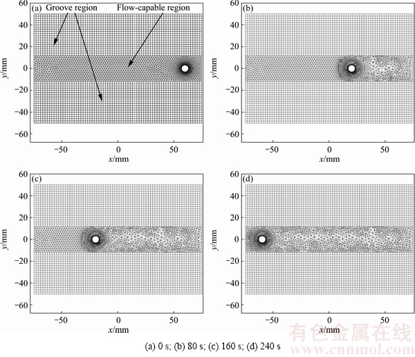
Fig. 2 Mesh plots showing re-meshing process during simulation of FSW

Similar conditions were maintained at different heights [19], despite the minor differences of temperature distribution and flow condition. Consequently, it was reasonable to complete the FSW simulation using a two-dimensional model.

It is extremely important to establish a reasonable thermal environment in the model. The heat input was achieved by setting the heat flux at the shoulder wall and pin walls in most three-dimensional models because the heat in FSW is created mainly by surface contact friction between the workpiece and tool. The workpiece surface that contacted with the tool was defined as the heat source, which contained three parts: a shoulder surface (SS), a pin side surface (PSS) and a pin bottom surface (PBS). The heat generated at the SS (Q_SS) is expressed as follows:

       (1)

where δ_SS is the contact state variable, which is assumed to be 0.35 in this study; ω is the tool angular velocity; R₁ is the radius of shoulder; R₂ is the top radius of the pin; τ_b is the maximum shear stress; r is the radius; μ is the coefficient of friction, which was 0.4; and P is the plunge pressure.

Due to different contact conditions, the contact state variable of PSS (δ_PSS) was assumed to be 0.5, and δ_PBS was set to be 0.35 according to the experiment. The Q_PSS and the Q_PBS are written as follows:

              (2)

       (3)

where R₃ is the bottom radius of the pin; h is the height variable; is the conic angle; H is the tool pin height; and P₁ is equal to the plunge pressure P.

The Q_PSS source was loaded on the circle wall, which was on the pin side in this model. However, there was not any wall to load the heat flux of the Q_SS and Q_PBS sources. Volumetric sources of energy (VSE) could be loaded in the source terms of the flow-capable region by the UDF code. VSE means loading the energy input from the volumetric cell, instead of the wall.

The heat flux (q_PSS) at the PSS can be expressed as follows:

              (4)

where R_M is the radius of the circle in the model, which is equal to 0.8R₁+0.2R₂ in this study.

The Q_SS and Q_PBS sources were translated to VSE in this model. VSE would be a moving source with the welding process at a speed of 30 mm/min, which was the same as the welding speed. VSE was a ring source under the tool shoulder between R_M and R₁ at which the energy was input. Considering the heat loss in the heat conduction from the contact surface, VSE received 80% of the energy of the Q_SS and Q_PBS, based on experience. Additionally, the source value in VSE was considered equal everywhere to simplify the calculation of the source, indicating that the energy was distributed uniformly in the source ring. The VSE source value V_VSE can be calculated by the equation as follows:

   (5)

The heat loss in the model is also important for a proper thermal environment. H_t is the heat dissipation coefficient on the workpiece side surfaces; in this study, H_t was 30 W/(m²·K). To balance the heat loss of the top surface and bottom surface, the value of H_t needed to be multiplied by the area ratio constant n (n=8.5), which is the ratio of the whole surface area to the side surface  area. H_t was defined in thermal boundary conditions of the side wall and was regarded as the only energy output in this two-dimensional model.

The thermal energy conservation equation is given as follows [20]:

       (6)

where c_p is the specific heat capacity, which is obtained by fitting the material property parameters; T is the temperature; μ_weld is the velocity in welding direction; x is the distance in every direction; k is the thermal conductivity of the weld material, which is obtained by fitting the material property parameters; S(θ) is the heat generation rate per unit area at the tool pin and workpiece interface; A_r is any arbitrarily selected area on the tool pin; and V is the volume over which the heat generated on A_r is dissipated.

In addition to the boundary conditions, the material properties have a large influence on the result of the simulation. The governing continuity equations for the material flow are given as follows:

                                    (7)

(8)

where u_i is the velocity of the material flow for i=1, 2, representing the x-direction and y-direction, respectively; ρ is the material density; P is the plunge pressure and η is the non-Newtonian viscosity.

The non-Newtonian viscosity, η, which is the most important parameter for fluid flow, is dependent on temperature and strain rate. It can be expressed as follows:

                                (9)

where σ is the flow stress; T is the temperature, which can be read via the fluent code; and  is the effective strain rate, which can be treated as the grid strain rate in the model [9].

Finally, the viscosity can be expressed as follows:

              (10)

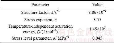
where α is the stress level parameter; n is the stress exponent; Q is the temperature-independent activation energy; R is the mole gas constant; and A is the structure factor. Equation (10) was loaded into the model by the UDF code. The relevant material parameters are presented in Table 1.

Zinc was also a material used in this study; however, zinc melts during the welding process when the temperature of the zinc exceeds 692 K (the melting point of zinc). The viscosity of the melted zinc was considered to be 0.001 kg/(m·s), similar to that of many other fluids, which was much less than that of the softened aluminum. However, this value was regarded to be 1×10⁶ kg/(m·s) when the temperature of the zinc got below 692 K, which was a proper value for the solid zinc in Fluent [19]. The special viscosity value of zinc was also loaded by the UDF code in the material properties.

Table 1 Material parameters of 6061 aluminum alloy

There are other different properties between these two materials, which have a substantial influence on the temperature distribution. The thermo-physical properties related to both materials are listed in Table 2.

4 Results and discussion

4.1 Temperature distribution and thermal environment

Figure 3 depicts the temperature distribution plot of the simulation plane at 180 s. During the modeling process, eight points were monitored to obtain the continuous T-T curves which can be compared with the experimental results.

The area around the tool reached the maximum temperature because the VSE source was input through this part, which replaced the energy created by the shoulder. The highest temperature was just above 754 K, and the lowest temperature was approximately 384 K. It should be noted that the region in front of the tool showed a higher temperature gradient than that behind it. The temperature between the advancing side and the retreating side was asymmetrical: the temperature on the advancing side was slightly higher than that on the retreating side, similar to most other experiments [13,20].

Table 2 Thermo-physical properties of 6061 aluminum alloy and zinc

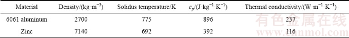
Fig. 3 Temperature contour plot of simulation plane at 180 s

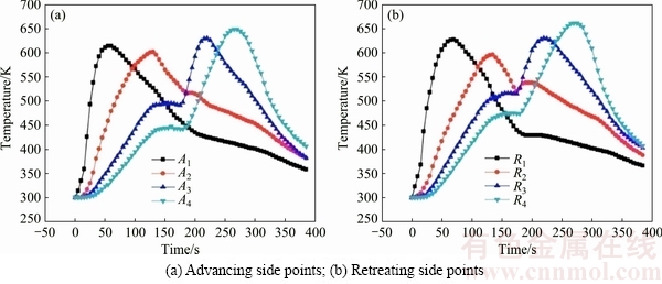
Fig. 4 Variation of transient temperature at given locations during FSW

Figure 4 shows the experimental temperature results measured by thermocouples. The temperatures of A₁, A₂, A₃ and A₄ points have a similar tendency to R₁, R₂, R₃ and R₄ points because of their symmetrical positions. However, there is a small difference between the peak temperatures of the two sides. The peak temperatures of the advancing side are slightly higher than those of the retreating side, as mentioned in earlier experiments. A_i and R_i are both regarded as point i (P_i) when discussing their tendency.

P₁ reached the peak temperature firstly (50 s), and P₄ reached the peak temperature lastly, but P₄ reached a higher peak temperature than P₁. This was because P₁ was closer to the start point than P₄ and was heated firstly. The temperature of P₁ increased rapidly and reached the peak temperature while other points were still at a very low temperature. When P₁ was heated, the temperatures of P₂, P₃ and P₄ started to increase slowly due to thermal conduction. Thus, P₄ was pre-heated when the rotating tool moved along the welding line; therefore, it had a higher temperature than the initial temperature [15]. When the tool arrived at the mid-points of A₄ and R₄, the same energy from contact friction was input. A higher original temperature caused P₄ to reach a higher peak temperature although thermal conduction always existed during the process to maintain the whole temperature field.

The peak temperature of P₂ was the lowest value among these four points (P₁, P₂, P₃ and P₄). The zinc stock melted completely during the movement of the tool from P₂ to P₃. The temperature around the tool exceeded 692 K, which was higher than that of P₂. The melting of zinc absorbed a significant amount of the energy created by friction. Additionally, the friction between the tool and the melted zinc decreased rapidly, which decreased the energy input directly. Eventually, P₂ did not reach  the same peak temperature as the other points. Simultaneously, P₃ and P₄ did not obtain enough energy to increase their temperatures in a short time as shown in their T-T curves. The temperature of the whole workpiece increased slowly from 120 to 180 s. The temperatures of P₃ and P₄ began to increase rapidly after this period. There is a small temperature resilience in P₂, which is caused by the solidification of melted zinc behind the tool. The zinc solidified when the temperature fell below 692 K. Latent heat of crystallization was liberated during the solidification to hold the temperature field for a short time.

The numerical simulation also produced the calculated result of the T-T curves, and the comparison between the simulation and the experiment is shown in Fig. 5. To achieve a reasonable conclusion, the start time point was defined as the moment that the tool started to move during the experiment, which was also 0 s in the simulation. The result of the retreating side was not shown in Fig. 5 because a similar conclusion was achieved with the advancing side.

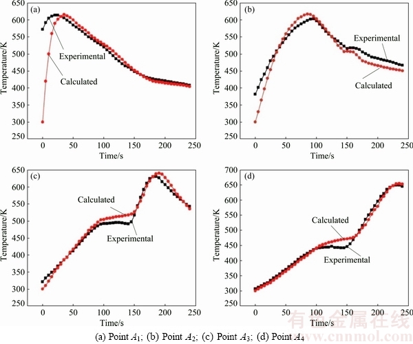
Fig. 5 Comparison between experimental and calculated temperatures of measured points

The workpiece was heated when the pin was plugged into it. It absorbed some energy before 0 s, meaning that the experimental results always had a higher initial temperature than the calculated results. The approximate peak temperatures were achieved almost simultaneously. It should be noted that the calculated results were higher than the experimental results by small errors that are within the permissible range, as shown in Figs. 5(b) and (c). The influence of zinc melting on the temperature distribution during the experiment is also shown in Fig. 5, where the melting process absorbed a substantial amount of energy and decreased the energy input from friction. However, the latter reason was in the calculated results because of the stable VSE source, which kept a constant energy heat input, even though the friction decreased during the experiment. The temperature resilience also exists in the calculated result of A₂ for the solidification of zinc, which agrees well with the experimental result.

These results show that the numerical model and the calculation method for heat generation are appropriate and that the thermal environment could be applied in further investigations.

4.2 Material flow behavior

The softened materials started to flow under the shearing force and pressure around them when the rotating tool approached or contacted them. However, it is too difficult to observe the flow behaviors directly during the FSW process. The simulation method was used to analyze the flow vectors and flow trajectories.

The flow trajectories combining with the flow vectors and flow streamtraces are depicted in Fig. 6. Streamtrace 1 showed that the softened material in front of the tool was driven to the retreating side with the rotation of the tool at a speed over 0.5 m/s under the shearing force. Simultaneously, the material on the advancing side was driven to the area in front of the tool. The vectors in front of the tool followed the tangential direction of the rotating tool. The other softened materials flowed under the shearing force from the flowing material in front of the tool, but there was not enough path to transfer them to the retreating side; thus they were extruded to the primary place rapidly. A small anticlockwise whirlpool formed on the retreating side in front of the tool during this process, as shown in Streamtrace 2. The rotating tool moved along the welding line, leaving an instantaneous cavity behind the tool, although a small amount of material entered from the retreating side, which caused a negative pressure in the area behind the tool [21]. The softened material behind the tool flowed following the direction of Streamtrace 1 under the negative pressure. Then, a small clockwise whirlpool, as shown in Streamtrace 3, formed behind the tool.

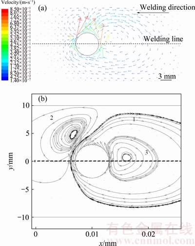
Fig. 6 Material flow vectors (a) and streamtraces (b) around tool

The zinc stock was embedded into the plate as a marker element to investigate the material flow in FSW. The zinc was also patched into the fluid region in the model as a second phase addition to the primary  material. Figure 7 depicts the instantaneous state when the rotating tool touched the patched zinc. The process of material flow that is highly consistent with the explanation of the streamtrace theory mentioned before is shown. The zinc was softened as the temperature approached 692 K. When temperature exceeded 692 K, zinc started to melt. Zinc close to the rotating tool was initially driven to the retreating side, and then, it flowed to the area behind the tool along Path 1. Whirlpools 2 and 3 formed under the positive and negative pressures previously mentioned. The whirlpools caused the melted zinc to mix uniformly with the primary material, and a joint with a uniform distribution of material was produced behind the tool.

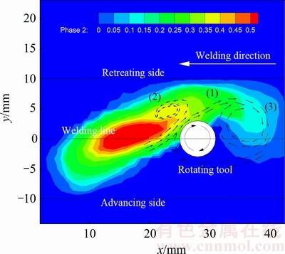
Fig. 7 Zinc flow behavior as second phase

A small part of the observing plane is displayed in Fig. 8. The zinc-enriched and the zinc-poor areas are distinguished clearly after slight corrosion in Figs. 8(a) and (b). The enriched zinc area is brighter than the zinc-poor area because the etchant corroded the aluminum alloy’s grain boundaries and dimmed the grains, but it brightened the zinc. Two types of grain forms are shown in Fig. 8(c) by magnifying the boundary Area A of Fig. 8(a). Figure 8(d) shows a magnified area of Area B in Fig. 8(b) where aluminum and zinc were evenly distributed.

The zinc was stirred evenly due to the clockwise whirlpool and a clear trajectory left behind the tool, as shown in Figs. 8(a) and (b). The area close to the welding line displayed long traces that were nearly perpendicular to the welding line, as shown in Fig. 8(a), following the same direction as that of Streamtrace 3 in Fig. 6(b). However, the area far away from the welding line on the retreating side showed serrated traces, as shown in Fig. 8(b). This finding was observed because the softened material moved along Streamtrace 1 in Fig. 6(b), and a part of the material precipitated if there was not enough pressure to drive it to move along the Streamtrace 3. The material precipitated repeatedly, forming the serrated traces in the retreating side.

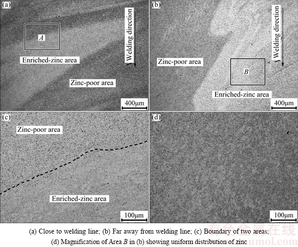
Fig. 8 Zinc distribution around welding line

5 Conclusions

1) The asymmetry of the temperature distribution during friction stir butt-welding of 6061 aluminum alloy determined by numerical simulation essentially corresponded with the results measured by the experiments. The peak temperatures on advancing side were 10 K higher than those on the retreating side.

2) The VSE source was shown to be available to heat the workpiece to its maximum temperature (754 K) combining with the side-wall radiating boundary condition. The region in front of the tool showed a higher temperature gradient than that behind it, which was a reasonable thermal environment in FSW.

3) Zinc was proved to be a proper marker material for both the experiment and numerical simulation in the butt-welding of 6061 aluminum alloy. The material flow behavior was clearly depicted by combining the two methods. The shearing force from the rotating tool drove the material to the retreating side behind the tool. There were three whirlpools formed under the special pressure environment, causing the composition distribution of the joint to be more uniform.

References

[1] THOMAS W M, NICHOLAS E D. Friction stir welding for the transportation industries [J]. Materials & Design, 1997, 18(4): 269-273.

[2] JOHNSEN M R. Friction stir welding takes off at Boeing [J]. Welding Journal, 1999, 78(2): 35-39.

[3] KISHORE V R, ARUN J, PADANABHAN R, BALASUB- RAMANIAN V. Parametric studies of dissimilar friction stir welding using computational fluid dynamics simulation [J]. The International Journal of Advanced Manufacturing Technology, 2015, 80(1-4): 91-98.

[4] ABNAR B, KAZEMINEZHAD M, KOKABI A H. Effects of heat input in friction stir welding on microstructure and mechanical properties of AA3003-H18 plates [J]. Transactions of Nonferrous Metals Society of China, 2015, 25(7): 2147-2155.

[5] DAWOOD H I, MOHAMMED K S, RAHMAT A, UDAY M B. Effect of small tool pin profiles on microstructures and mechanical properties of 6061 aluminum alloy by friction stir welding [J]. Transactions of Nonferrous Metals Society of China, 2015, 25(9): 2856-2865.

[6] SATO Y S, URATA M, KOKAWA H. Parameters controlling microstructure and hardness during friction-stir welding of precipitation-hardenable aluminum alloy 6063 [J]. Metallurgical and Materials Transactions A, 2002, 33(3): 625-635.

[7] HEJAZI I, MIRSALEHI S E. Mechanical and metallurgical characterization of AA6061 friction stir welded joints using microhardness map [J]. Transactions of Nonferrous Metals Society of China, 2016, 26(9): 2313-2319.

[8] KIRAL B G, TABANOGLU M, SERINDAG H T. Finite element modeling of friction stir welding in aluminum alloys joint [J]. Mathematical and Computational Applications, 2013, 18(2): 122-131.

[9] GEMME F, VERREMAN Y, DUBOURG L, JAHAZI M. Numerical analysis of the dwell phase in friction stir welding and comparison with experimental data [J]. Materials Science and Engineering A, 2010, 527(16): 4152-4160.

[10] ZHANG Zhao, ZHANG Hong-wai. Numerical studies on the effect of transverse speed in friction stir welding [J]. Materials & Design, 2009, 30(3): 900-907.

[11] COX C, LAMMLEIN D, STRAUSS A, COOK G. Modeling the control of an elevated tool temperature and the effects on axial force during friction stir welding [J]. Materials and Manufacturing Processes, 2010, 25(10-12): 1278-1282.

[12] NAIDU R. Friction stir welding: Thermal effects of a parametric study on butt and lap welds [D]. Wichita: Wichita State University, 2006.

[13] YADUWANSHI D K, BAG S, PAL S. Numerical modeling and experimental investigation on plasma-assisted hybrid friction stir welding of dissimilar materials [J]. Materials & Design, 2016, 92: 166-183.

[14] ZHANG Jing-qing, SHEN Yi-fu, LI Bo, XU Hai-sheng, YAO Xin, KUANG Bin-bin, GAO Ji-cheng. Numerical simulation and experimental investigation on friction stir welding of 6061-T6 aluminum alloy [J]. Materials & Design, 2014, 60: 94-101.

[15] PASHAZADEH H, TEIMOURNEZHAD J, MASOUMI A. Numerical investigation on the mechanical, thermal, metallurgical and material flow characteristics in friction stir welding of copper sheets with experimental verification [J]. Materials & Design, 2014, 55: 619-632.

[16] ZHAO Yan-hua, LIN San-bao, HE Zi-qiu, WU Lin. Microhardness prediction in friction stir welding of 2014 aluminium alloy [J]. Science and Technology of Welding and Joining, 2006, 11(2): 178-182.

[17] BHATTACHARYA T K, DAS H, PAL T K. Influence of welding parameters on material flow, mechanical property and intermetallic characterization of friction stir welded AA6063 to HCP copper dissimilar butt joint without offset [J]. Transactions of Nonferrous Metals Society of China, 2015, 25(9): 2833-2846.

[18] SWAIN S, MOHANTY S. A 3-dimensional Eulerian–Eulerian CFD simulation of a hydrocyclone [J]. Applied Mathematical Modelling, 2013, 37(5): 2921-2932.

[19] HE Xixo-cong, GU Feng-shou, BALL A. A review of numerical analysis of friction stir welding [J]. Progress in Materials Science, 2014, 65: 1-66.

[20] NANDAN R, ROY G G, DEBROY T. Numerical simulation of three-dimensional heat transfer and plastic flow during friction stir welding [J]. Metallurgical and Materials Transactions A, 2006, 37(4): 1247-1259.

[21] MENDEZ P F, TELLO K E, LIENERT T J. Scaling of coupled heat transfer and plastic deformation around the pin in friction stir welding [J]. Acta Materialia, 2010, 58(18): 6012-6026.

6061铝合金搅拌摩擦对接焊的数值模拟

赵鹏程，沈以赴，黄国强，郑其贤

南京航空航天大学 材料科学与技术学院，南京 210016

摘  要：建立计算流体动力学二维模型模拟6061铝合金的搅拌摩擦对接焊。运用动网格，使模型中的搅拌针能像实验中的搅拌针一样水平移动和绕轴转动，而且体热源能为模型提供一个与实验相似的温度场。另外，将一小块锌嵌入被焊工件中，作为示踪元素研究焊接流动行为。通过数值模拟，得到焊接过程的温度分布和矢量分布图。通过实验的温度监控以及金相分析，间接证明了模拟结果的合理性。模拟结果表明，焊缝两侧的温度分布并不对称，但具有相同的变化趋势，且前进侧的峰值温度比后退侧高约10 K。迹线图和相分布图反映焊接过程的流动性。在搅拌针转动剪切力和前进挤压作用下，搅拌针周围形成3种运动涡流，这些涡流使得搅拌针周围材料搅拌更加剧烈，成分分布更加均匀。

关键词：铝合金；搅拌摩擦焊；数值模拟；动网格；示踪元素法；温度分布；涡流

(Edited by Wei-ping CHEN)

Foundation item: Project (51475232) supported by the National Natural Science Foundation of China

Corresponding author: Yi-fu SHEN; Tel: +86-25-84895940; E-mail: yfshen_nuaa@hotmail.com

DOI: 10.1016/S1003-6326(18)64759-4