J. Cent. South Univ. (2016) 23: 644-653

DOI: 10.1007/s11771-016-3110-4

Capacity analysis of inhomogeneous hybrid wireless networks using directional antennas

WU Feng(吴丰)¹, ZHU Jiang(朱江)¹, TIAN Yi-long(田毅龙)², ZOU Jian-bin(邹建彬)¹

1. School of Information Science and Engineering, National University of Defense Technology,

Changsha 430074, China;

2. School of Computer, National University of Defense Technology, Changsha 430074, China

 Central South University Press and Springer-Verlag Berlin Heidelberg 2016

Abstract: Most of studies on network capacity are based on the assumption that all the nodes are uniformly distributed, which means that the networks are characterized by homogeneity. However, many realistic networks exhibit inhomogeneity due to natural and man-made reasons. In this work, the capacity of inhomogeneous hybrid networks with directional antennas for the first time is studied. By setting different node distribution probabilities, the whole network can be devided into dense cells and sparse cells. On this basis, an inhomogeneous hybrid network model is proposed. The network can exhibit significant inhomogeneity due to the coexistence of two types of cells. Then, we derive the network capacity and maximize the capacity under different channel allocation schemes. Finally, how the network parameters influence the network capacity is analyzed. It is found that if there are plenty of base stations, the per-node throughput can achieve constant order, and if the beamwidth of directional antenna is small enough, the network capacity can scale.

Key words: network capacity; hybrid networks; inhomogeneity; directional antennas; infrastructure; ad hoc networks

1 Introduction

Network capacity has been extensively studied in recent years. There are two obvious reasons explaining why so many researchers engage in this pursuit. First, network capacity reflects the asymptotic behavior of the wireless networks. In face of the emerging large-scale networks, asymptotic capacity of the networks becomes more critical. Second, regardless of detailed protocol, network capacity focuses on the prediction of network performance as a function of the number of nodes in the network. In contrast, simulation or numerical results are deterministic as they can only be obtained for a fixed number of nodes. Besides, the simulation or numerical results are available after considering all the details and it may cost a lot, such as time and computing resource. Therefore, capacity is one of the most important properties in wireless networks. Nevertheless, it is also a challenging work.

In the seminal work, Gupta and Kumar [1] studied the asymptotic capacity of large scale wireless networks. They proved that the throughput capacity is  which means that the transmission rate of per-node decreases at the speed of  as the number of nodes increases, and finally it will decrease to zero as n goes to infinity, where n is the number of nodes. Later, extensive studies have been conducted to achieve a tighter capacity bound [2-6]. Franceschetti et al [2] applied percolation theory to obtain a per-node transmission rate higher than  Grossglauser and Tse [3] proved that the mobility of ad hoc nodes can increase the network capacity. They show that per-node transmission rate of  can be achieved when ad hoc nodes are mobile, while the transmission delay will go to infinity.

Hybrid networks, where base stations are added to help the transmissions of ad hoc nodes, have attracted many researchers’ attention in recent years [7-10]. Liu et al [7] studied the capacity of hybrid networks where base stations are placed in a regular pattern. They showed that the asymptotic behavior of m makes the hybrid networks exhibit different capacities, where m denotes the number of base stations. Kozat and TASSIULAS [8] considered the case that base stations are randomly deployed. They concluded that base stations can improve the per-node throughput capacity significantly. Zemlianov and VECIANA [9] proposed a hybrid network model where base stations are arbitrarily placed. They derived the network capacity and got similar conclusions.

To the best of our knowledge, most of the researches on capacity of hybrid networks are based on the assumption that ad hoc nodes are uniformly distributed in the area, which means that their network models are characterized by homogeneity. Nevertheless, in most real cases, networks exhibit inhomogeneity [11-12]. A few works have analyzed the capacity of inhomogeneous networks [13-17]. In Refs. [13-14], a network model is proposed where n nodes wish to communicate with m cluster head. However, the overall node density does not exhibit inhomogeneity. PEREVALOV et al [15] studied the capacity of a clustered wireless network. ALFANO et al [16-17] proposed a network model where nodes are placed according to a shot-noise Cox process (SNCP) and obtained the capacity bounds.

Furthermore, some researchers studied the capacity of networks where directional antennas are used [18-21]. As using directional antennas obtains a higher spatial ratio and reduces the interference area caused by nodes in the networks, network capacity can be obviously improved. Yi et al [18] analyzed the capacity improvement when directional antennas are used. They showed that the capacity gain is  when both transmission and reception are directional. Zhang et al [19] studied the capacity of wireless mesh networks with directional antennas. They considered about the case that there is only one gateway in the network and all nodes’ traffic goes through the gateway. ZHANG et al [20] studied the capacity of hybrid networks with directional antennas under L-maximum-hop resource allocation. They analyzed the impact of some important parameters on the capacity of hybrid networks.

In this work, we study the capacity of inhomogeneous hybrid networks with directional antennas equipped for each node. In our model, base stations divide the whole area into several cells. We focus on the difference of node density of each cell due to natural and man-made reasons (such as landform, urban or suburban settlement). By setting different spatial distribution probabilities for each cell, we divide the cells into two types: dense cells and sparse cells. The network can exhibit significant inhomogeneity when dense cells and sparse cells coexist.

Based on the network model, we study the throughput capacity of dense cells and sparse cells separately. Then, we derive the capacity of the whole networks and obtain the maximum capacity under different channel allocation schemes. Besides, we analyze the impact of some important parameters such as the number of sparse cells and the beamwidth of directional antennas on the per-node throughput capacity. Finally, we get some interesting conclusions which could guide the network design. Compared with the previous literature, the main contributions of this work are as follows.

We propose an inhomogeneous hybrid network model where all the nodes are equipped with directional antennas. By setting different spatial distribution probabilities, we divide the cells into dense cells and sparse cells. The coexistence of the two types of cells makes the network exhibit significant inhomogeneity.

We derive the capacity of the inhomogeneous hybrid networks with directional antennas. Compared with the homogeneous hybrid network, we find that insignificant inhomogeneity does not change the capacity of the whole network.

We analyze the influence of some important network parameters to the per-node throughput capacity of the network. We find that if the number of base stations is large enough, the per-node throughput can achieve constant order, and if the beamwidth is small enough, the capacity of network can scale.

Notations: the following notations are used throughout this work. Given f(n) and g(n), there are

1)  means that there exists a positive c and m such that  and for all n≥m;

2)  means that there exists a positive c and m such that  and for all n≥m, namely,

3) means that both   and  hold;

4)  means

2 Network model

2.1 Network architecture

We consider a hybrid wireless network with n ad hoc nodes and m base stations in a unit disk. As shown in Fig. 1, we assume that the base stations are regularly deployed. Hence, the unit area is divided into m hexagon cells. Each base stations lies in the center of the cell where it is and a wired network connects all the base stations. Furthermore, the base stations are just as relay nodes, which only work in routing and transmission to other ad hoc nodes.

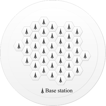
Fig. 1 Hybrid network model

To model the inhomogeneous node spatial distribution, we divide the distribution process of ad hoc nodes into two steps. Firstly, n nodes are deployed into each cell according to different distribution probabilities. For node i (1≤i≤n), the probability that it is located in cell k (1≤k≤m) is p_k, so we have  Then, for the nodes in a certain cell, they are independent and identically distributed (i.i.d.). Though the distribution of nodes in a certain cell is homogeneous, the overall node spatial distribution is inhomogeneous.

Specially, when p₁=p₂=…=p_m=1/m, our model is the same as the homogeneous hybrid network model. In other words, the homogeneous hybrid networks can be taken as a particular case of our model.

2.2 Directional antenna model

There are more than twenty types of antennas in the antenna family, which can be grouped under omnidirectional and directional [21]. Here, we adopt a directional antenna model as shown in Fig. 2. Each directional antenna is modeled as a circular sector. Let r denote the radius of the circular sector and θ denote the angle. The radius r represents the communication range of each node and the angle θ represents the beamwidth of the directional antenna. Although the side lobes of realistic antennas are ignored in this model, the idealization of directional model will make little sense to the results of our work [20].

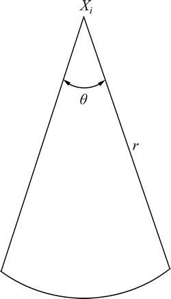
Fig. 2 Directional antenna model

Due to the inhomogeneous node density of cells, it is unnecessary to ensure that all nodes have the same transmission distance. We assume that there are N_k nodes in cell k and the transmission distance of node X_i in cell k is r_k. Let a circle C(s_i, r_k) centered at point s_i with radius r_k represent the area node where X_i can cover. To ensure the connectivity of the whole network, the N_k nodes should satisfy  where D_k denotes the region of cell k. We also set r_max=max{r₁, r₂, …, r_m}, r_min=min{r₁, r₂, …, r_m}, and r_max/r_min=α. For simplicity, we assume that the beamwidths of all the directional antennas are the same, namely. all the nodes have the same angle θ.

According to the transmission and the reception schemes with the use of directional antennas, wireless networks can be classified into four categories: directional transmission and directional reception (DTDR), omnidirectional transmission and omnidirectional reception (OTOR), directional transmission and omnidirectional reception (DTOR), omnidirectional transmission and directional reception (OTDR) [22]. In this work, we only consider about the DTDR networks, namely. directional antennas work in both transmission and reception. The capacity of the other three types of networks can be easily obtained in a similar method which we will deploy later.

2.3 Communication model

Now we consider about the communication model using directional antennas. Considering the influence of directional antennas to the transmission and reception, we propose a directional antenna based communication model, as shown in Fig. 3.

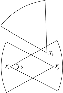
Fig. 3 Communication model

In cell k, node X_j can receive the transmission from node X_i successfully if the following conditions hold:

1) Node X_j is within the transmission distance of node X_i, i.e.

                                (1)

2) For every other node X_t which is simultaneously delivering packets,

                         (2)

where Δ_k defines the size of guard zone of cell k. Due to the inhomogeneity of node density, the size of guard zone of a cell may be different from that of others. For simplicity, we set:  

2.4 Routing strategy

Routing strategies can be divided into two types in hybrid networks: infrastructure mode and ad hoc mode. In infrastructure mode, packets from source node are delivered to the destination through base stations, which is applied to long distance transmissions. In ad hoc mode, the transmission process only relies on the relay nodes, which is applied to short distance transmissions.

In this work, we use the 0-nearest-cell routing strategy proposed in Ref. [9]. If the source node and the destination node are in the same cell, they communicate in ad hoc mode. If they are in different cells, they communicate in infrastructure mode.

We assume that each node is capable of transmitting at W bits/s (bits per second). In cell k, we assign the bandwidth W into W₁, W₂ and W₃, denoting the intra-cell, uplink and downlink sub-channel respectively, then W₁+W₂+W₃=W. For simplicity, we let W₂=W₃.

2.5 Capacity definition

In Ref. [9], the capacity analysis is based on the aggregate throughput capacity of the whole network instead of a single node. We extend this definition to our network model.

Definition 1: Feasible aggregate throughput. For a network, if there is a temporal and spatial scheduling scheme that yields a per-node throughput of λ(n) bits/s on average, and an aggregate throughput of T(n)=nλ(n) bits/s, we say the aggregate throughput of T(n) is feasible.

Definition 2: Aggregate throughput capacity. The aggregate throughput capacity is of order O(f(n)) bits/s if there is a deterministic constant c₁<+∞ such that

           (3)

And is of order  if there are deterministic constants 0<c₂<c₃<+∞ such that

          (4)

           (5)

3 Throughput capacity of inhomogeneous hybrid wireless networks using directional antennas

3.1 Dense cells and sparse cells

Consider cell k, let Y_i denote whether node i (1≤i≤n) and its destination node are both in cell k. Y_i is defined as

                                (6)

For every node in the network, the probability that it is located in cell k is p_k, hence we get  Then, let where N_k denotes the number of source-destination pairs in cell k. Since the distribution of nodes in each cell is i.i.d., the sequence  is i.i.d.. By strong law of large numbers, we have:

                  (7)

Here, we consider two cases:  and If we have:  and if is bounded by a constant. According to the asymptotic behavior of p_k, we divide all the cells into dense cells and sparse cells.

Definition 3: Dense cell. For cell k, if the node distribution probability  we say that cell k is a dense cell.

Definition 4: Sparse cell. For cell l, if the node distribution probability  we say that cell l is a sparse cell.

Definition 5: Insignificant inhomogeneity. For a hybrid network, we say that its inhomogeneity is insignificant if there exists only one type of cell in the network. Otherwise, its inhomogeneity is significant.

The number of dense cells is related to the total number of cells, i.e. the number of base stations. For simplicity, we set that cells 1, 2, …, l are dense cells and cells l+1, …, m are sparse cells. Let m_d denote the number of dense cells and m_s denote the number of sparse cells, i.e. m_d=1 and m_s=m-l. The following lemma shows the relationship of m_d and m.

Lemma 1: If  we have m_d≥1, namely, if m grows slower than  there is at least one dense cells. And if  we have  namely, if m grows faster than  the number of dense cells is constrained or zero.

Proof: According to the definition of dense cells and sparse cells, we have:

Let  and  then, we have

 and

Given  we have

It can also be written as

Since  and  we get  If  similarly,  is bounded by a constant. So, we have

There are two special cases we should note. The first case is that the number of the base stations is small and there exist only dense cells in the network, i.e. both  and m_d=m hold. The second case is that there are plenty of base stations and all the cells are sparse cells, i.e. both  and m_s=m hold. In these two cases, the hybrid networks exhibit insignificant inhomogeneity.

3.2 Aggregate capacity

There are three different sub-channels in the network: the intra-cell, uplink and downlink sub-channels, denoted by W₁, W₂ and W₃, respectively. For simplicity, we assume there is no interference between them. What we consider about is the interference between two intra-cell sub-channels of two neighboring cells. A lot of works have proved that the interference between two intra-cell sub-channels is bounded by a constant factor in a homogeneous network. However, in an inhomogeneous network, the transmission ranges of the nodes in different cells are not the same, which is different from the homogeneous network model studied before. To solve this problem, we redefine the interfering neighbors of a cell and obtain a similar conclusion to other literature, i.e. the interference between two intra-cell sub-channels is also limited in an inhomogeneous network. Now, we provide the formal proof.

Definition 6: Interfering neighbors. For a point in cell l, if there is another point in cell k satisfying that the distance of the two points is less than  we say cell l and cell k are interfering neighbors.

Lemma 2: For any cell in the network, the number of its interfering neighbors is limited by a constant c, which only depends on α and △_max.

Proof: Let a denote the length of each cell (hexagon). For arbitrary cell k, we assume that a=b_kr_k, where b_k s a constant. Therefore, cell k contains a disk with radius  and is contained by a disk with radius b_kr_k.

For an arbitrary interfering neighbor of cell k, let o' denote its center. By the definition of interfering neighbor, the distance of o' and o is no further than  where o is the center of cell k. Therefore, all the interfering neighbors of cell k must be contained by a disk with radius

Considering the directional antennas, the probabilities that nodes interfere with each other is θ²/(4π²). Thus, we can derive that the number of interfering neighbors is loosely bounded by

                  (8)

By Lemma 2, we can conclude that there is a spatial scheduling policy that each cell gets one slot to transmit data in every (1+c) slots.

In the following passage we calculate the aggregate capacity of our network model. Considering an inhomogeneous hybrid network with several dense cells and sparse cells, we firstly analyze the capacity of dense cells and the capacity of sparse cells in ad hoc mode.

Theorem 1: With directional antennas, the throughput capacity of a dense cell k () contributed by ad hoc mode is

  (9)

Proof: Given we have  the number of source-destination pairs  According to Theorem 1 in Ref. [18], with directional antennas, the throughput capacity of per-node is

Hence, the aggregate capacity of cell k is

By Eq. (7), we get that the aggregate capacity of a dense cell k is

Theorem 2: With directional antennas, the throughput capacity of sparse cell l () contributed by ad hoc mode is

                          (10)

Proof: Given  as n goes to infinity, the number of nodes in cell l is constrained. Therefore, the method in Theorem 1 does not apply to the sparse cell to derive the capacity.

According to the conclusion of Ref. [18], if n nodes are optimally distributed in a fixed area, the transport capacity of the network with directional antennas is

 bit-meters/sec

where λ denotes the highest transmission rate of per-node and L denotes the average distance between the source and destination of a packet.

In our network model, the m base stations are regularly placed in the unit area, hence the area of each cell is A=1/m and  Obviously, the transport capacity Eq. (2) gives is larger than that of a random network, hence we obtain the aggregate capacity of the sparse cell l in our model:

                    (11)

So, we have:

               (12)

Theorem 1 and Theorem 2 have given the throughput capacity of dense cells and sparse cells contributed by ad hoc mode, now we derive the aggregate capacity of the whole networks. We consider two cases: the networks characterized by significant inhomogeneity and the networks characterized by insignificant inhomogeneity. For the first types of networks, both dense cells and sparse cells exist in the networks, i.e. m_d≠0 and m_s≠0 For the second types of networks, only one type of cells (dense cells or sparse cells) exists in the network, i.e. m_d=0 or m_s=0. The following theorems will give the capacity of the two types of networks.

Theorem 3: If the network exhibits significant inhomogeneity, i.e. both m_d≠0 and m_s≠0 hold, its aggregate capacity is

                                        (13)

where

Proof: Since there is no inference between different types of sub-channels, the aggregate capacity of the whole network is  where is the aggregate capacity contributed by infrastructure mode and  is contributed by ad hoc mode.

As the base stations are connected by a wired network, we think the bandwidths of base stations are not constrained. Hence, they will not be the bottleneck in the transmission process. Therefore, the aggregate capacity of the whole network contributed by infrastructure mode is

                           (14)

Now, we calculate the capacity contributed by ad hoc mode. In our network model, the network consists of dense cells and sparse cells. For simplicity, we assume that cell k is a dense cell and cell l  is a sparse cell. By Theorem 1 and Theorem 2, the aggregate capacity contributed by ad hoc mode is

                        (15)

Let  According to L' Hospital rule, when n goes to infinity, Eq. (14) can be simplified as

               (16)

According to Eq. (16), if n goes to infinity,  is a linear function, hence we have:

     (17)

As  we get

                    (18)

By Eqs. (17)-(18), the aggregate capacity contributed by ad hoc mode is

        (19)

Combining Eqs. (14) and (19), we can obtain the aggregate capacity of the whole network

 (20)

Theorem 4: For a hybrid network using directional antennas characterized by insignificant inhomogeneity (m_d=0 or m_s=0), if all the cells are dense cells, the aggregate capacity is:

                 (21)

And if all the cells are sparse cells, the aggregate capacity is

                       (22)

Proof: If all the cells are dense cells, we have p=1 and m_d=m, by Theorem 3, we can obtain the aggregate capacity is

And if all the cells are sparse cells, we have p=0 and m_d=0. Based on the analysis above, the aggregate capacity is

Theorem 4 gives the capacity of the networks characterized by insignificant inhomogeneity, note that Eqs. (21)-(22) do not include the parameters m_d and m_s, we can conclude that insignificant inhomogeneity does not change the capacity of the whole networks.

4 Capacity analysis

In this section we analyze how the network parameters influence the throughput capacity. We will obtain the maximum capacity of the network under different channel allocation schemes. On the basis, we analyze how the number of sparse cells and the angle of directional antennas θ affect the capacity of the networks.

4.1 Capacity under different channel allocation schemes

In the above sections, the bandwidth W is divided into W₁, W₂ and W₃ without considering the inhomogeneous node density of each cell. Now, we derive the maximum capacity of the network under different channel allocation schemes.

Without loss of generality, we assume that dense cells and sparse cells coexist in the network, the capacity is

For dense cells, we assign the bandwidth W to W_d1, W_d2 and W_d3, denoting intra-cell, uplink and downlink sub-channels respectively. Similarly, for sparse cells, we assign the bandwidth W to W_s1, W_s2 and W_s3. Then, we have W=W_d1+W_d2+W_d3= W_s1+W_s2+W_s3.

The following corollary gives the maximum capacity when different channel allocation schemes are used.

Corollary 1: If  and  the capacity of the inhomogeneous hybrid networks with directional antennas can be maximized as

           (23)

Proof: By Theorem 3, Eq. (23) can be written as

                                 (24)

          (25)

               (26)

where T_d denotes the aggregate capacity of all the dense cells in the network and T_s denotes the aggregate capacity of all the sparse cells. To get the maximum capacity, we should maximize T_d and T_s, separately.

Since W_d2=W_d3, we have

                              (27)

Substitute Eq. (26) into Eq. (23), we have

 (28)

For dense cells, because  and  we have:  and  For directional antennas, we have  Therefore, when n is large enough, we have:

                       (29)

We can obtain the maximum capacity of dense cells if :

                   (30)

For a sparse cell l, the aggregate capacity is

                   (31)

Since  the aggregate capacity of cell l is maximized when  the maximum capacity of cell l is

                     (32)

And the maximum capacity of all the sparse cells in the network is

                             (33)

Combining Eqs. (30)-(33), under different channel allocation schemes, the maximum capacity is

           (34)

Corollary 1 implies that in order to achieve the maximum capacity, different channel allocation schemes should be applied in different cells. In dense cells, more bandwidth should be assigned to carry the intra-cell traffic. And in sparse cells, we should assign more channel bandwidth to carry inter-cell traffic.

4.2 Parameters analysis

Based on the conclusion of Corollary 1, we will analyze the influence of network parameters to the per-node throughput capacity in the following passage.

Figure 4 shows the relationship between the number of sparse cells and the aggregate throughput capacity of the whole networks. Let  denote the maximum throughput of per-node, now we analyze the relationship between m_s and the per-node throughput  We have the following conclusions.

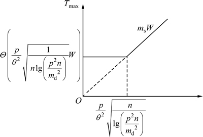
Fig. 4 relationship between m_s and aggregate throughput capacity

If  the maximum aggregate capacity of the whole network is  hence the maximum throughput of per-node is:

                  (35)

It means that if the number of sparse cells is large enough, i.e.  the per-node throughput is of constant order and the network can scale.

If  the maximum aggregate capacity is hence the maximum per-node throughput is

               (36)

which means that in this case the per-node throughput decreases to zero as n goes to infinity and the network can not scale.

Now, we discuss how the angle of directional antennas θ influences the capacity of per-node. Figure 5 shows the relationship between the directional antenna angle θ and the aggregate throughput capacity.

Ifthe maximum aggregate capacity is

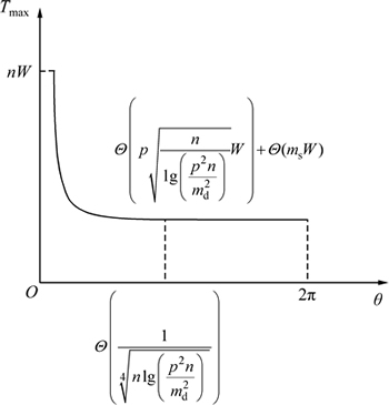
Fig. 5 relationship between antenna angle and aggregate throughput capacity

                    (37)

Hence, the maximum per-node throughput is

                  (38)

The analysis above implies that the per-node throughput capacity is improved as the beamwidth of directional antenna θ becomes smaller. If the beamwidth is smaller enough, the per-node throughput capacity will be large enough until it achieves a constant not exceeding W/2, and in this case the network can scale.

If we have  as n goes to infinity. As  the analysis implies that if the antenna beamwith is large, it will not affect the throughput capacity significantly, and then the main factors which influence the per-node throughput are the number of dense cells m_d and the number of nodes n. In this case the throughput of per-node will decrease as the number of nodes goes large, and the network can not scale.

5 Conclusions

In this work, we have studied the throughput capacity of inhomogeneous hybrid networks with directional antennas. By setting different node distribution probabilities for the cells, the networks can exhibit significant inhomogeneity. We have derived the aggregate capacity of the network and obtain the maximum capacity under different channel allocation schemes. On this basis, we have analyzed the influence of network parameters to the network capacity. We prove that when  the throughput capacity of per-node can be  regardless of what value other parameters can take. We also find that if the beamwidth of directional antennas is small enough, the network can scale.

References

[1] GUPTA P, KUMAR P R. The capacity of wireless networks [J]. IEEE Transactions on Information Theory, 2000, 46(2): 388-404.

[2] FRANCESCHETTI M, DOUSE D, TSE D, THIRAN P. Closing the gap in the capacity of random wireless networks via percolation theory [J]. IEEE Transactions on Information Theory, 2007, 53(3): 1009-1018.

[3] GROSSGLAUSER M, TSE D. Mobility increases the capacity of ad hoc wireless networks [J]. IEEE/ACM Transactions on Networking, 2002, 10(4): 477-486.

[4] JIANG Chun-xiao, CHEN Yan, REN Yong, LIU K J R. Maximizing network capacity with optimal source selection: A network science perspective [J]. IEEE Signal Processing Letters, 2015, 22(7): 938-942.

[5] ZHANG Guang-lin, XU You-yun, WANG Xin-bing, GUIZANI M. Multicast capacity for hybrid vanets with directional antenna and delay constraint [J]. IEEE Journal on Selected Area in Communications, 2012, 30(4): 818-833.

[6] HUANG Tao, TENG Ying-lei, LIU Meng-ting, LIU Jiang. Capacity analysis for cognitive heterogeneous network with idea/non-idea sensing [J]. Frontiers of Information Technology & Electronic Engineering, 2015, 16(1): 1-11.

[7] LIU Ben-yuan, LIU Zhen, TOWSLEY D. On the capacity of hybrid wireless networks [C]// Proceedings of IEEE INFOCOM. San Francisco. USA: IEEE, 2003: 1543-1552.

[8] KOZAT U C, TASSIULAS L. Throughput capacity of random ad hoc networks with infrastructure support [C]// Proceedings of ACM Mobi Com. San Diego, USA, 2003: 55-65.

[9] ZEMLIAVOV A, VECIANA G. Capacity of ad hoc wireless networks with infrastructure support [J]. IEEE Journal on Selected Areas in Communications, 2005, 23(3): 657-667.

[10] LIN Chen. Throughput capacity of multi-channel hybrid wireless network with antenna support [J]. Applied Mathematics & Information Science, 2014, 8(3): 1455-1460.

[11] SUN Ning, JEONG Yoon-su, LEE Sang-ho. Energy efficient mechanism using flexible medium access control protocol for hybrid wireless sensor networks [J]. Journal of Central South University, 2013, 20(8): 2165-2174.

[12] CAI Zi-xing, WEN Sha, LIU Li-jue. Dynamic cluster member selection method for multi-target tracking in wireless sensor network [J]. Journal of Central South University, 2014, 21(2): 636-645.

[13] TOUMPIS S. Capacity bounds for three types of wireless networks: Asymmetric, cluster and hybrid [C]// Proceedings of ACM Mobi Hoc. Roppongi, Japan: ACM, 2004: 133-144.

[14] KULKARNI S R, VISWANATH P. A deterministic approach to throughput scaling in wireless networks [J]. IEEE Transactions on Information Theory, 2004, 50(6): 1041-1049.

[15] PEREVALOV E, BLUM R S, SAFI D. Capacity of clustered ad hoc networks: How large is large? [J]. IEEE Transactions on Communication, 2006, 54(9): 1672-1681.

[16] ALFANO G, GARETTO M, LEONARDI E. Capacity scaling of wireless networks with inhomogeneous node density: Upper bounds [J]. IEEE Journal on Selected Areas in Communications, 2009, 27(7): 1147-1157.

[17] ALFANO G, GARETTO M, LEONARDI E, MARTINA V. Capacity scaling of wireless networks with inhomogeneous node density: Lower bounds [J]. IEEE/ACM Transactions on Networking, 2010, 18(5): 1624-1636.

[18] YI Su, PEI Yong, KALYANARAMAN S. How is the capacity of ad hoc networks improved with directional antennas? [J]. Wireless Networks, 2007, 13(5): 635-648.

[19] ZHANG Jun, JIA Xiao-hua, ZHOU Yuan. Analysis of capacity improvement by directional antennas in wireless sensor networks [J]. ACM Transactions on Sensor Networks, 2012, 9(1). doi>10.1145/2379799.2379802

[20] ZHANG Guang-lin, XU You-yun, WANG Xin-bing, GUIZANI M. Capacity of hybrid networks with directional antenna and delay constraint [J]. IEEE Transactions on Communications, 2010, 58(7): 2097-2106.

[21] KRAUS J D, MARHEFKA J. Antennas: for all applications [M]. 3rd ed. New York: McGraw-Hill, 2002.

[22] LI Pan, ZHANG Chi, FANG Yu-guang. The capacity of wireless Ad Hoc networks using directional antennas [J]. IEEE Transactions on Mobile Computing, 2011, 10(10): 1374-1387.

(Edited by DENG Lü-xiang)

Foundation item: Projects (61401476, 61201166) supported by the National Natural Science Foundation of China

Received date: 2015-05-26; Accepted date: 2015-09-08

Corresponding author: WU Feng, PhD; Tel: +86-13317376405; E-mail: wufengpaper@163.com