Trans. Nonferrous Met. Soc. China 25(2015) 3381-3388

Construction and solution of strain model along thickness of aluminum alloy plate under plastic deformation

Shu-yuan ZHANG^1,2, Kai LIAO¹, Yun-xin WU²

1. School of Mechanical and Electrical Engineering, Central South University of Forestry and Technology, Changsha 410004, China;

2. School of Mechanical and Electrical Engineering, Central South University, Changsha 410083, China

Received 21 November 2014; accepted 12 May 2015

Abstract: A thickness strain model of aluminium alloy plate under plastic deformation, based on thin plate assumption was proposed. It is found that when ratio of stress fractions is constant during in-plane loading, ratios of strain components under various loading conditions are linearly related and these points of ratios form a η-η line. Under these simple loadings, strains in thickness direction can be easily calculated by the η-η line equation without integral and differential work. When the plate is under more complicated loading conditions, the thickness can be computed by the proposed optimization and piecewise calculation model. Validation computations indicate that the relative error of the results of the presented model is less than 0.75% compared with the proven theories and FE simulation. Therefore, the developed model can be applied to engineering calculation, e.g. pre-stretching analysis of aerospace aluminium thick plate, with acceptable accuracy.

Key words: isotropic linear hardening; thick plate; strain model; plastic deformation; aluminum alloy

1 Introduction

7000 series aluminum alloy thick plates are widely applied in aerospace for their combination of high strength, stress-corrosion-cracking resistance and toughness. Stretching is a typical process performed on solid solution treated aluminum thick plate to release quenching-caused residual stresses through leading uniform deformation to the plate in the rolling direction [1].

Since available and measurable variables in stretching process are strains of the plate, it is reasonable to establish the analytical model based on strain-space plasticity theory, which originated from soil and rock mechanics. DRUCKER [2] firstly considered the possibility of formulating the theory of elasto-plastic material in strain space. The studies performed by NAGHDI, TRAPP and CASEY [3,4] contributed to the establishment of the theory by using plastic strain as state variables with which most researchers are familiar. YODER and IWAN [5] employed the relaxation stress as state variables in formulations of strain space plasticity. HAN and CHEN [6] built strain-space plasticity formulation for hardening-softening materials with elasto-plastic coupling, while FARAHAT et al [7] modeled for concrete with compressive hardening- softening behavior in strain-space. LU and VAZIR [8] claimed that the stress- and strain-based plasticity theories are equivalent by offering the alternative conjugate expressions for the loading criteria, provided that the material laws used are identical in both approaches.

The tensile tests performed on AA7075-T6 and 2024-T3 by LEE and SHAUE [9] indicated that the materials are linear hardening. The compressive tests under quasi-static loading conducted by ABOTULA and CHALIVENDRA [10]  and WU et al [11] showed the similar stress-strain relations. Although mechanical properties in the rolling and transverse directions of commercial wrought aluminum alloy are slightly different, the material can be considered to be isotropic for simplification of modeling.

The aluminum thick plate is in plane-stress state during stretching and in-plane stresses of it vary along the thickness-direction [1,12]. As is used in stress measurement methods, such as layer removal [13,14], incremental hole drilling [15], layer X-ray method [16] and crack compliance method [17], thick plate can be virtually divided into many thin sheets along its thickness-direction and stress evolution in the thick plate can be deduced from the stress status of the separated thin sheets by superposition which was described in Ref. [18]. Since the thickness of the virtually divided thin sheet in the thick plate cannot be measured directly, a model, which relates strain in the thickness-direction to strains in the rolling/transverse direction, is the basis for the research on residual stresses in the thick plate.

At present, the model for calculating thickness of metallic plate under in-plane deformation is still relatively lacking. Researches concerned with the evolution of plate’s thickness are mostly focused on bending deformation. ZHU [19] studied large deformation pure bending of the wide plate made of the power-law-hardening material. The results showed that large curvature bending leads to a significant thickness reduction of the bent plate. COLLIE et al [20] used analytical models, numerical models and elastic–plastic FEA to predict the final deformed geometry of induction bends in thick-walled pipe. PENG et al [21] established a theoretical solution to thickness variation of bending metal sheet with perfect plasticity and linear hardening character. In general, researches concerning theory of plate/shell or non-linear plate theory [22] do not give solution of thickness-direction strain of thin plate under in-plane deformation and there are no models can be applied to calculating strain of thickness-direction z for aluminum plate which is under in-plane deformation directly. With this model, the thickness of plate can be computed by knowing deformation in the rolling and the transverse directions.

2 Plate-layered hypotheses

Residual stresses in the aluminum thick plate is relieved by applying a uniform plastic strain on it [23] and a schematic diagram of stretching process for the plate is shown in Fig. 1. The plate is under uniaxial tension load which is uniformly distributed at each end of the plate along the rolling direction (x-direction) while quenching- caused residual stress σ_r, varies along the thickness- direction. Since the length and the width are much larger than the thickness, the thick plate is in-plane stress during the stretching process. In order to obtain stress state at a given depth, the thick plate is assumed to be made up of N layers of thin plates and one of them is depicted in dash line in Fig. 1. The thin plate has a tiny thickness, e.g., less than 1/40 of thickness of the thick plate, so that the in-plane stress of it can be considered as constant throughout its thickness. By knowing the stress status of these thin plates, the stress evolution of the thick plate can be easily deduced.

The loading condition of the thin plate is also drawn in Fig. 1. The thin plate, with the same length and width as the thick plate, is under uniformly distributed loads, F_x and F_y, in the rolling and the transverse directions respectively. F_x and F_y are caused by the material around the thin plate during stretching. With the increase of F_x and F_y, stresses of the thin plate will grow from initial state to the stress of elastic limit σ_x. After that, the thin plate will deform plastically under further loading.

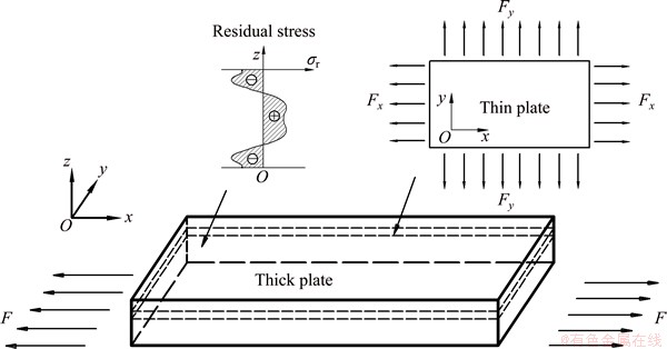
Fig. 1 Schematic depiction of aluminium alloy plate to be stretched and thin plate under in-plane deformation

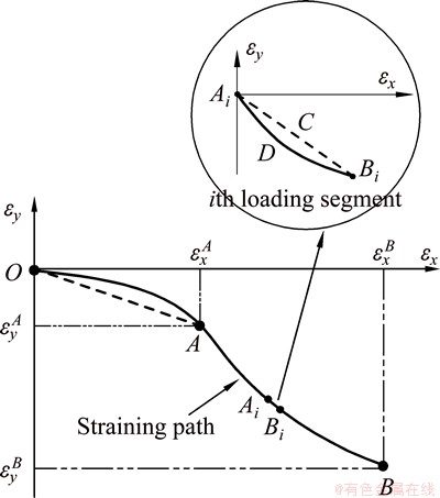
Fig. 2 Strain evolution of thin plate during stretching

Figure 2 shows the evolution of the thin plate’s strain state in the x and y directions during deformation. In the plot, the abscissa ε_x is strain component in the rolling direction and the ordinate ε_y is strain in the transverse direction. The straining path of the thin plate is nonlinear and drawn in solid line in Fig. 2. The original state before deformation is defined as Point O while Point A refers to the state when deformation of the thin plate reaches the yield limit. The terminal of loading is Point B and the thin plate is straining plastically during stage AB.

Since the loading stage OA is elastic straining, the stress status at Point A can be deduced by knowing strains at Point A and the loading path can be considered as the straight dash line between Point O and Point A. However, the stress status at Point B depends on the plastic loading path from Point A to Point B. In order to calculate the nonlinear straining path AB, the path is divided into enormous linear loading segments because it is easier to calculate the liner loading than nonlinear one. A loading section, the ith loading segment, is also depicted in Fig. 2. Since the segment A_iDB_i is fairly short, it can be regarded as straight line A_iCB_i in computation with acceptable accuracy. Therefore, the first step of calculation is to establish a model for linear loading during plastic deformation and then develop a model for nonlinear plastic loading.

It is supposed that the straining path between Points A and B is straight line. Thus, incremental strain fractions are linearly related to each other in the deformation stage of OA and AB, the relations between the strain increments are then expressed as

                       (1)

where  and  are proportion factors during OA and AB stages, respectively. The superscript OA and AB of η_yx indicate that the variable is about the corresponding stage. Meanwhile, the superscripts of strain ε_ij indicate that the variable is an increment from Point O to Point A or from Point A to Point B , e.g.,  and .

If factor  is not constant in deformation stage AB, i.e., the straining path is nonlinear loading shown in solid line in Fig. 2, the stage will be divided into a number of short loading segments, such as segment A_iB_i in Fig. 2, and η_yx of each segment is nearly invariable when the number of segments is large enough. Then, the model for linear loading can be applied to the given deformation segment when Point A and Point B are designated as the start and the end of it.

3 Construction of strain calculation model

In order to establish a model for ε_z under in-plane deformation, relations between (ε_x, ε_y) and ε_z under given loading conditions are established by numerical computation. The linear loading condition will be discussed first and then the more complicated nonlinear loading.

3.1 Consistent of stress increment ratio

From the deformation theory of plasticity, it is clear that the relation between strain components remain invariable when the proportion between stress components is constant. Thus, the linear straining condition can be obtained by presetting a linear stress loading path because strain increment in terms of stress increment has been well established and proved for isotropic hardening material. In this case, a thin plate is assumed under linear loading during plastic deformation and thus the proportion between stress fractions in the x and y directions of it is constant from the deformation theory of plasticity, i.e.,

γ_yx=σ_y/σ_x                                    (2)

where γ_yx remains invariable during loading from Point O to Point B. In stress space, the yield function of the isotropic hardening material can be expressed as

                     (3)

where  is the accumulated plastic strain, k is the hardening function, and J₂ is the second invariant of the stress deviator tensor. Based on the flow rule, the Hooke’s law and the consistency condition, the expression of the strain increment [24] is

              (4)

where D_ijkl is the tensor of elastic compliance, h is the plastic modulus and σ_kl is the stress increment. Without loss of generality, the material properties are Poisson ratio υ=0.33, elastic modulus E=1, slope of hardening     line E_t=1/11, stress of elasticity limit σ_s=1 and plastic

modulus = 0.1E.

Suppose γ_yx=3 and then the stress history of the thin plate is from O (0, 0, 0) to B (3, 9, 0). Substituting parameters in Table 1 into Eqs. (3) and (4) and Hooke’s law, the evolution of strain components can be calculated and the results are shown in Fig. 3.

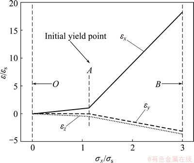
Fig. 3 Evolution of strain components during loading

In Fig. 3, the turning points of the three lines correspond to the initial yield Point A in Fig. 2. It can be found that all strain components grow linearly from Point A to Point B, indicating that strain ratio  is a constant. Besides, the ratio of incremental strain components between the z and x directions, i.e., , is invariable in AB stage. From strain curves shown in Fig. 3, the connection between ε_z and ε_x or ε_y is still unclear.

However, considering that ratios of strain components are constant, a relation between  and  under different γ_yx is expected. Therefore, it is assumed that the values of γ_yx are -10¹⁰, -20, -5, -1, -0.5, 0, 0.5, 1, 10, 20 and 10¹⁰, respectively, the above computation is repeated while supposing . The calculation results are drawn in Fig. 4.

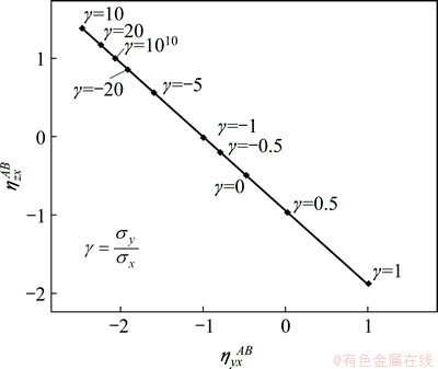
Fig. 4 Relation of ratios between strain components under various loading conditions

From Fig. 4, it is clear that all points corresponding to different γ_yx lie on a straight line. Thus, a conclusion can be drawn that  and  have a linear relationship when the ratio of stress fractions γ_yx is constant during loading.  can be easily calculated by equation of the line, which is named η-η line for simplicity. Since uniaxial loading meets the requirements of point on the η-η line, the line’s equation can be determined by the values of  and  under uniaxial tensions in the x and y directions, respectively.

In the case of uniaxial tensile loading in the rolling direction, the ratios of strain components can be calculated by using Eq. (4):

                        (5)

Similarly, the ratios of strain components under uniaxial transverse loading are

,                       (6)

In view of Eqs. (5) and (6), the equation of η-η line can be expressed as

                    (7)

3.2 Inconsistent of stress increment ratio

In the case of more complicated loading, i.e., , ratios of strain components are nonlinearly related to each other and the accurate value of  cannot be obtained by Eq. (7).

It is assumed that stress increase during loading stage AB is fairly small, e.g., σ_x^AB=10^-3σ_s, then components of σ^AB can be treated as being linearly related. Two loading paths are then concerned: (-0.5, 0.3) and . Using the same method applied in Fig. 4 and the parameters in Table 1, the strain ratios during AB stage of the above two paths are drawn in Fig. 5 in comparison with points on η-η line.

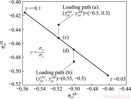
Fig. 5 Relation of ratios between strain fractions under two loading paths

In Fig. 5, the abscissa of points (c) and (d) are equal to that of points (a) and (b), respectively. In order to calculate the stress corresponding to loading paths (a)-(d), a counterpart of Eq. (4) in strain space, i.e. the strain-based elastic-plastic incremental constitutive model, is employed and a general expression of it is

                 (8)

where Q is the plastic potential function, F is the yield function in strain space, A is a scale factor. Substituting the material properties and strains relation to the loading paths (a)-(d) in Fig. 4 into Eq. (8), σ_z^AB of the corresponding paths can be computed and there are relations as follows:

         (9)

Since σ_z^AB is zero under plane stress, the values of  at points (a) and (b) are more accurate than those of points (c) and (d). In view of relations in Eq. (9), an optimization rule for  can be deduced and it is shown in Fig. 6.

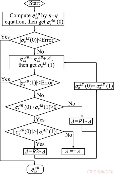
Fig. 6 Flow chart of optimization for

4 Validation and discussion with FEM

A FEM analysis is performed by using FE software MSC.Marc and the result of simulation is compared with that of η-η method. Actual material parameters of Al7075 used both in simulation and calculation are Poisson ratio υ=0.33, elastic modulus E=69.5 GPa, slope of hardening line E_t=3 GPa, stress of elasticity limit σ_s=410 MPa and plastic modulus

=3135 MPa.

The numerical simulation model is based on the specimen, of which the dimensions are 1200 mm × 220 mm × 50 mm, measured by LIAO et al [25]. Since the geometry and the boundary conditions are symmetrical, a simplification of the FE model is applied by using 1/8 of the plate to reduce the calculation time required. A numerical thin plate model with dimensions of 600 mm ×110 mm × 2.5 mm is established in MSC.Marc according to the specimen and it is illustrated in Fig. 7, and then the model is divided into 10 layers. An 8-node 3D solid element of 10 mm × 10 mm × 0.5 mm is selected in each layer. Stress and strain of thin plate with 3D entity deformation were calculated by this model. Two adjacent edges of thin plate are fixed, and uniform displacement is exerted on the other two edges according to loading parameter. Boundary conditions above mentioned the model calculation conditions are the same.

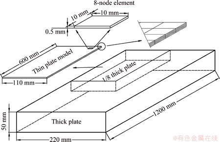
Fig. 7 FE model of thin plate used in simulation

4.1 η-η method

It is assumed that  and σ_x^AB = σ_s /2, the stress of the thin plate increased from Point O (0, 0, 0) to Point B (652.34 MPa, 130.47 MPa, 0) during loading. The results of simulation and η-η calculation are compared in Fig. 8. It can be found that the result of η-η matches the FE result very well.

Compared with Eq. (4) and FE simulation, η-η line equation is much simpler and easier to be used in engineering application for its markedly reduced calculation without integration and differential work.

4.2 Optimization method

When , the optimization and piecewise (OP) method described in Fig. 6 is applied to calculating the z-direction strain.

In the first place, a calculation flow, here named σ-ε-σ, is used to testify the accuracy of the algorithms with the material being applied. The loading conditions in terms of stress are preset firstly and Eq. (4) is used to calculate the corresponding strain evolutions under these loadings. Then, the results of computed strain are applied to the calculation flows in Fig. 6 to obtain the stress data which are compared with the preset stresses. The preset loading conditions in terms of stress and the results of computation are listed in Table 1.

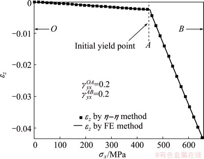
Fig. 8 Computed z-direction strain of thin plate by η-η method in comparison with results of FE simulation

Table 1 Parameters and results of σ-ε-σ validation

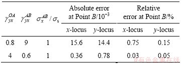
The stress growth in the x direction during plastic deformation, , is σ_s under these loadings and is divided into 20 segments in the piecewise method. The maximum number of iteration cycles in optimization method is 50 and the initial step length of searching, Δ, is 1% of , which is calculated by η-η method. The strain evolutions, calculated by Eq. (4), from Point A to Pint B corresponding to the loading paths are listed in Table 1. The computation results are described in Fig. 9.

It is clear in Fig. 9 that the computed stresses are in good agreement with the preset stresses. Table 1 shows that the maximum relative error is below 0.75%, indicating that OP method has an acceptable accuracy. If the number of segments and iteration cycles increases, better accuracy would be obtained. In the simulation validation, the second loading path listed in Table 1 is applied to the FE model illustrated in Fig. 9. The results of the simulation and the OP method are shown in Fig. 10.

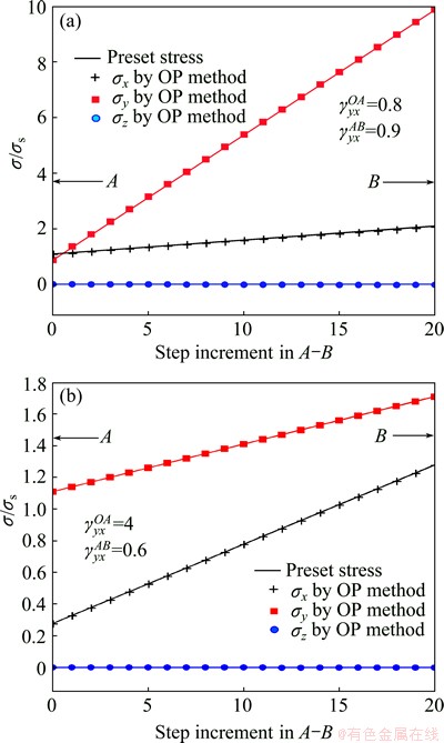
Fig. 9 Computed stress curves by OP method in comparison with preset stress

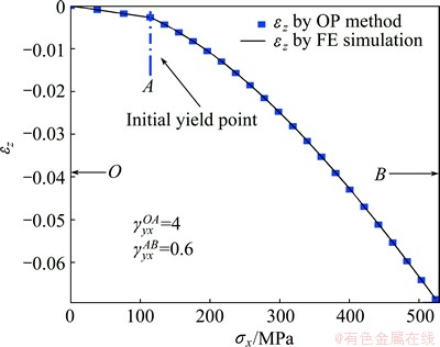
Fig. 10 Comparison between computed z-direction strains by OP method and FE simulation for thin plate under second loading path in Table 1

Figure 10 shows that the calculated thickness-direction strain matches the results of FE analysis very well. The comparison of the results suggests that the developed calculation model has a good accuracy when the plastic deformation stage is finely meshed. Since the model is developed under strain hardening background, the developed model, η-η and OP method can also be applied to computing the thickness of plate made by perfect plastic material, such as steel. The model developed above has been applied to the research, described in Ref. [18], on the residual stress in stretched aluminum plate.

5 Conclusions

1) When ratio of stress fractions is constant during in-plane loading, ratios of strain components (, ), under various loading conditions are linearly related and these points of ratios form a η-η line. In the case of simple loading, strains in thickness direction can be easily calculated by the η-η line equation without integral and differential calculation.

2) When the plate is under more complicated loading conditions, the thickness of the plate can be computed by the proposed optimization and piecewise calculation model after dividing its plastic deformation stage into short loading segments. Validation computations indicate that the results of the presented model are in good agreement with those of the proven theory and FE simulation. Therefore, the developed model can be applied to engineering calculation with acceptable accuracy.

References

[1] PRIME M B, HILL M R. Residual stress, stress relief, and inhomogeneity in aluminum plate [J]. Scripta Materialia, 2002, 46: 77-82.

[2] DRUCKER D C. Some implications of work hardening and ideal plasticity [J]. Quarterly Journal of Applied Mathematics, 1950, 7(4): 411-418.

[3] NAGHDI P M, TRAPP J A. The significance of formulating plasticity theory with reference to loading surfaces in strain space [J]. International Journal of Engineering Science, 1975, 13(9-10): 785-797.

[4] CASEY J, NAGHDI P M. On the nonequivalence of the stress space and strain space formulations of plasticity theory [J]. ASME Journal of Applied Mechanics, 1983, 50(2): 350-354.

[5] YODER P J, IWAN W D. On the formulations of strain space plasticity with multiple loading surfaces [J]. ASME Journal of Applied Mechanics, 1981, 48(4): 773-778.

[6] HAN D J, CHEN W F. Strain-space plasticity formulation for hardening-softening materials with elastoplastic coupling [J]. International Journal of Solids and Structures, 1986, 22(8): 935-950.

[7] FARAHAT A M, KAWAKAMI M, OHTSU S M. Strain-space plasticity model for the compressive hardening-softening behavior of concrete [J]. Construction and Building Materials, 1995, 9(1): 45-59.

[8] LU P F, VAZIRI R. The equivalence of stress- and strain-based plasticity theories [J]. Computer Methods in Applied Mechanics and Engineering, 1997, 147: 125-138.

[9] LEE H T, SHAUE G H. The thermomechanical behavior for aluminum alloy under uniaxial tensile loading [J]. Materials Science and Engineering A, 1999, 268: 154-164.

[10] ABOTULA S, CHALIVENDRA V B. An experimental and numerical investigation of the static and dynamic constitutive behavior of aluminium alloys [J]. The Journal of Strain Analysis for Engineering Design, 2010, 45: 555-565.

[11] WU Y F, LI S H, HOU B, YU Z Q. Dynamic flow stress characteristics and constitutive model of aluminum 7075-T651 [J]. The Chinese Journal of Nonferrous Metals, 2013, 23(3): 658-665.

[12] PRIME M B. Residual stress measurement by successive extension of a slot: The crack compliance method [J]. Applied Mechanics Reviews, 1999, 52(2): 75-96.

[13] WANG Shu-hong, ZUO Dun-wen, WANG Min, WANG Zong-rong. Modified layer removal method for measurement of residual stress distribution in thick pre-stretched aluminum plate [J]. Transactions of Nanjing University of Aeronautics & Astronautics, 2004, 21(4): 286-290.

[14] BENDEKA E, LIRAA I, FRANC-OISB M, VIAL C. Uncertainty of residual stresses measurement by layer removal [J]. International Journal of Mechanical Sciences, 2006, 48: 1429-1438.

[15] PRIME M B, MICHAEL R H. Uncertainty analysis, model error, and order selection for series-expanded, residual-stress inverse solutions [J]. Journal of Engineering Materials and Technology, 2006, 11: 175-185.

[16] HU Yong-hui, WU Yun-xin, CHEN Lei, GUO Jun-kang. Experimental measurement of surface residual stresses of quenched aluminum alloy thick plate by X-ray method [J]. Materials China, 2011, 30(2): 51-55. (in Chinese)

[17] GONG Hai, WU Yun-xin, LIAO Kai. Analysis on validity of residual stress measurement methods for aluminum alloy thick-plate [J]. Journal of Materials Engineering, 2010(1): 42-46. (in Chinese)

[18] ZHANG S Y, WU Y X, GONG H. A modeling of residual stress in stretched aluminum alloy plate [J]. Journal of Materials Processing Technology, 2012, 212: 2463-2473.

[19] ZHU H X. Large deformation pure bending of an elastic plastic power-law-hardening wide plate: Analysis and application [J]. International Journal of Mechanical Sciences, 2007, 49: 500-514.

[20] COLLIE G J, HIGGINS R J, BLACK I. Modelling and predicting the deformed geometry of thick-walled pipes subjected to induction bending [J]. Journal of Materials: Design and Applications, 2010, 224: 177-189.

[21] PENG Y R, JIANG Y, DUAN J C, ZHAO F, LUO W B. A theoretical solution to thickness variation of bending metal sheet with perfect plasticity and linear hardening character [J]. Journal of Plasticity Engineering, 2003, 10(3): 22-25.

[22] STEIGMANN D J. Thin-plate theory for large elastic deformations [J]. International Journal of Non-linear Mechanics, 2007, 42: 233-240.

[23] TANNER D A, ROBINSON J S. Modelling stress reduction techniques of cold compression and stretching in wrought aluminium alloy products [J]. Finite Elements in Analysis and Design, 2003, 39(5-6): 369-386.

[24] CHEN W F, SALEEB A F. Elasticity and plasticity [M]. Beijing: China Architecture & Building Press, 2005.

[25] LIAO Kai, WU Yun-xin, GONG Hai, YAN Peng-fei, GUO Jun-kang. Effect of non-uniform stress characteristics on stress measurement in specimen [J]. Transactions of Nonferrous Metals Society of China, 2010, 20(5): 789-794.

塑性变形下铝合金板材厚向应变模型的构建和求解

张舒原 ^1,2，廖 凯 ¹，吴运新²

1. 中南林业科技大学 机电工程学院，长沙 410004；

2. 中南大学 机电工程学院，长沙 410083

摘  要：建立适合铝合金材料的各向同性线性强化薄板在平面应力状态下塑性变形时厚向应变的求解模型。当加载于薄板的应力分量之比在平面内塑性变形过程中为常数时，薄板的应变分量间呈线性关系，研究发现这一系列不同应力比例和对应的应变比例值构成直线方程，即η-η线。因此，当应力分量间呈恒比例关系加载于薄板时，其厚度方向的应变可以通过η-η线方程快速得到，避免了积分和微分运算。当薄板处于更加复杂的加载状态时，其厚度可以通过提出的迭代优化算法模型得到。研究表明，计算结果与现有理论和有限元仿真结果的相对误差小于0.75%，其精度达到工程应用要求。该模型可用于航空高强铝合金厚板预拉伸工艺分析等实际应用。

关键词：各向同性线性硬化；厚板；应变模型；塑性变形；铝合金

(Edited by Xiang-qun LI)

Foundation item: Project (51475483) supported by the National Natural Science Foundation of China; Project (2014FJ3002) supported by Science and Technology Project of Hunan Province, China; Project supported by Aid Program for Science and Technology Innovative Research Team in Higher Educational Institutions of Hunan Province, China

Corresponding author: Kai LIAO; Tel: +86-731-85623381; E-mail: liaokai102@163.com

DOI: 10.1016/S1003-6326(15)63973-5