J. Cent. South Univ. (2019) 26: 168-183

DOI: https://doi.org/10.1007/s11771-019-3991-0

Modeling and application of thermal contact resistance of ball screws

GAO Xiang-sheng(高相胜)¹, WANG Min(王民)^{1, 2}, LIU Xue-bin(刘学滨)¹

1. Beijing Key Laboratory of Advanced Manufacturing Technology, College of Mechanical Engineering and

Applied Electronics Technology, Beijing University of Technology, Beijing 100124, China;

2. Beijing Key Laboratory of Electrical Discharge Machining Technology, Beijing 100191, China

Central South University Press and Springer-Verlag GmbH Germany, part of Springer Nature 2019

Abstract: Aiming at determining the thermal contact resistance of ball screws, a new analytical method combining the minimum excess principle with the MB fractal theory is proposed to estimate thermal contact resistance of ball screws considering microscopic fractal characteristics of contact surfaces. The minimum excess principle is employed for normal stress analysis. Moreover, the MB fractal theory is adopted for thermal contact resistance. The effectiveness of the proposed method is validated by self-designed experiment. The comparison between theoretical and experimental results demonstrates that thermal contact resistance of ball screws can be obtained by the proposed method. On this basis, effects of fractal parameters on thermal contact resistance of ball screws are discussed. Moreover, effects of the axial load on thermal contact resistance of ball screws are also analyzed. The conclusion can be drawn that the thermal contact resistance decreases along with the fractal dimension D increase and it increases along with the scale parameter G increase, and thermal contact resistance of ball screws is retained almost constant along with axial load increase before the preload of the right nut turns into zero in value. The application of the proposed method is also conducted and validated by the temperature measurement on a self-designed test bed.

Key words: ball screw; fractal theory; thermal contact resistance; contact stress; preload

Cite this article as: GAO Xiang-sheng, WANG Min, LIU Xue-bin. Modeling and application of thermal contact resistance of ball screws [J]. Journal of Central South University, 2019, 26(1): 168–183. DOI: https://doi.org/ 10.1007/s11771-019-3991-0.

1 Introduction

Ball screws, popular transmission components, are widely used in machine tools, robots, measuring instruments and automatic equipment due to advantages in precise positioning and high efficiency [1]. However, a high amount of heat is produced due to friction during the continuous rotation of ball screws, causing a temperature rise and consequently leading to thermal errors. This would finally deteriorate the positioning accuracy of feeding systems [2]. Among the factors affecting deformations, the deformation induced by thermal expansion constitutes a high proportion, especially in precision and ultra-precision machining [3]. During thermal deformation prediction, the thermal characteristic of the key interface requires to be introduced to the ball screw mechanism (BSM) system. Modeling of thermal contact resistance of ball screws is the key problem in thermal deformation evaluation. Many studies have been conducted on the thermal contact resistance of ball screws.

LI et al [4] considered that the friction heat generation from the bearing and ball screw pairs is the main heat source. The coupled thermo- mechanical deformation analysis was conducted on the platform of finite element analysis (FEA) software with consideration to thermal contact resistance. MIN et al [5] determined the thermal contact resistance between the bearing and the corresponding housing by the work of BOSSMANNS et al [6] and developed an integrated thermal model with the aid of finite element method for temperature distribution analysis of a ball screw feed drive system. JIN et al [7] conducted thermal error predictions and compensations of a ball screw feed system under various operating conditions. In the research, the thermal contact resistance between the balls and both the inner and outer rings of the supporting bearing was determined by Hertz theory and JHM method (Jones-Harris method), but the thermal contact resistance of ball screws was obtained without the microscopic characteristics of the contact surfaces considered in the aforementioned research.

MB fractal theory is an effective method to solve thermal contact resistance of rough surfaces with microscopic fractal characteristics of the interfaces considered. JIANG et al [8] presented a fractal model for analyzing the thermal contact resistance (TCR) of rough surfaces. The relation for the TCR in terms of contact load was obtained for heat conductive surfaces with known material properties and surface topography. The analytical results were validated by aforementioned experiments. The recursive tree thermal contact resistance model based on the Cantor set fractal theory was obtained in Ref. [9]. The topography of rough contact surfaces was described with the Cantor set fractal theory. Moreover, an elastic- plastic theory was developed for the deformation of surface asperities to be obtained, where the volume conservation of plastic deformation was considered. A random number model based on fractal geometry theory was developed in Ref. [10] for the thermal contact conductance (TCC) calculation of two rough surfaces in contact. The present study presents that fractal parameters D and G have important effects on TCC. LIU et al [11] proposed a thermal resistance network model of spindle-bearing-bearing pedestal based on the fractal and Hertz contact theory. Effects of thermal contact resistance and thermal-conduction resistance were considered. MB fractal theory was adopted on the premise of contact stress distribution. Hertz theory was widely used for contact status analysis [12], and the thermal contact conductance was obtained [13–18]. But for ball screws, the raceway in ball screws, nut-raceway and screw-raceway, is not a toroid. They are 3D surfaces with spiral characteristics owing to the lead angle. The contact region is asymmetrical. The greater the lead angle leads to the more asymmetrical the contact region. Hertz theory can be only applied in symmetrical or axisymmetric contact surface. Relatively large errors will occur when Hertz theory is applied.

Therefore, a new analytical method combining the minimum excess principle with the MB fractal theory is proposed for thermal contact resistance estimation of ball screws in this research. The calculating flowchart of thermal contact resistance estimation of ball screws is depicted in Figure 1. Firstly, a geometrical shape of the contact surfaces in ball screws is analyzed; the parameter equations regarding screw-raceway and nut-raceway are established. The 3D contact surfaces of raceways are simulated and meshed based on the parameter equations. Secondly, the normal contact stress is solved by the minimum excess principle. Fast Fourier transform (FFT) is adopted for the convolution solution, and used in effects of normal stress on deformation in the normal direction evaluation. The conjugate gradient method is employed for the contact model solution. Finally, the thermal contact resistance of the diminutive areas is obtained by the MB fractal theory. The thermal contact resistance of ball screws is determined according to the series or parallel connections among them further. Microscopic fractal characteristics of joints could be considered in this research. The effectiveness of the proposed method is also validated by the self-designed experiment. Furthermore, effects of the fractal parameters and axial load on the thermal contact resistance of ball screws are discussed. The application of the proposed method in a finite element model of ball screws is also conducted and validated by the temperature measurement in a self-designed test bed in this research.

Figure 1 Flowchart of thermal contact resistance estimation

2 Modeling

2.1 Geometrical shape of contact surfaces

The lead angles of the screw-raceway and nut-raceway are different, due to the pitch being the same and the arc radius being different. The geometrical shape of contact surfaces is determined by lead angle and arc radius of raceways, thread angle and diameter of balls. The coordinate system at the contact points is established to describe the accurate geometrical shapes of contact surfaces.

The Cartesian coordinates AX_AY_AZ_A and BX_BY_BZ_B depicted in Figure 2 are established at the contact point (A) between the screw-raceway and the ball, and the contact point (B) between the nut-raceway and the ball, respectively. A and B are the initial contact points. In this situation, no normal stress exists. Both the Z_A-axis and Z_B-axis are perpendicular to the tangent plane at the contact points. Both the X_A-axis and X_B-axis are parallel to the tangential direction t of the center track of the balls. The Y_A-axis and Y_B-axis are both determined by the right-hand rule.

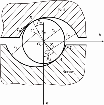
Figure 2 Ball screw coordinates

The parameter equations of the ball surfaces are the same because of the symmetry of balls, which are described as follows.

k=A, B             (1)

The geometrical shape of the contact surfaces at the coordinates (AX_AY_AZ_A) and (BX_BY_BZ_B) established at the A and B can be obtained by coordinate transformation.

is the arc parameter equation in the cross section of the screw-raceway at contact point A of the Frenet-Serret coordinate system[19, 20] O_Htnb, which is given by

,

               (2)

where r_s is the arc radius in the cross section of screw-raceway; r_b is the radius of balls; β_A is the thread angle between the ball and screw-raceway, β_AS is the central angle corresponding to the arc in the cross section of the screw-raceway, β_A0 is used to define the variation of the central angle β_AS.

In the same way, , the parameter equation of the arc in the cross section of the nut-raceway at contact point B of the Frenet-Serret coordinate system O_Htnb, is given by:

              (3)

where r_N is the radius of the arc in the cross section of the nut-raceway; β_B is the thread angle between the ball and nut raceway; β_BS is the central angle corresponding to the arc in the cross section of the nut-raceway; β_B0 is used to define the central angle β_BS variation.

According to coordinate transformations, the equations of raceway (2) and (3) are expressed as follows:

(4)

 (5)

where andare parameter equations of the arc in the cross section of the nut-raceway at contact points A and B of the coordinate system OXYZ;represents the coordinate transformation matrix from the coordinate system OXYZ attached to the screw, to the Frenet-Serret coordinate O_Htnb established at the track of the balls.is given by:

From Figure 2,andthe coordinate transformation matrices from the coordinate O_Htnb to the AX_AY_AZ_A and BX_BY_BZ_B, can be obtained respectively.

        (6)

        (7)

andequations of arcs in the screw- raceway and nut-raceway in the coordinate systems AX_AY_AZ_A and BX_BY_BZ_B, can be obtained from Eqs. (4)–(7).

               (8)

,

              (9)

whereis the coordinate transformation matrix at θ=θ_C. θ_C is the central angle corresponding to the helix at the A or B contact point where the ball/raceway contact occurs.

The geometrical shape of the contact surfaces in the coordinate systems AX_AY_AZ_A and BX_BY_BZ_B can be obtained by this method where β_AS or β_BS is assigned to different values. The variation of β_AS or β_BS is given in Eqs. (8)–(9) and the variation of θ is θ_C–θ₀≤θ≤θ_C+θ₀.

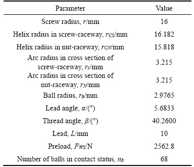
In this paper, a certain type of ball screw is studied. Parameters of the ball screw are listed in Table 1.

Table 1 Ball screw parameters

The geometrical shape of the raceways in ball screws can be obtained by Eqs. (8)–(9), which is depicted in Figure 3. The geometrical shape will be taken into account in the normal stress analysis. It is necessary for contact stress and thermal contact resistance analysis.

2.2 Normal stress analysis

The minimum excess principle is employed for the contact status solution of ball/raceway in ball screws. The contact problem is described as variational inequality to solve the minimum excess, depicted by the product of force and displacement. The method is suitable for analyzing contact problems with irregular contact surfaces [21, 22].

2.2.1 Discretization of contact region

The region near contact points should be meshed in order for numerical solutions of the normal contact stress to be obtained. A coordinate system OXY is established on the tangent plane of two contact bodies at A(B). The normal contact stress in the contact region is parallel to the Z-axis of the OXY system.

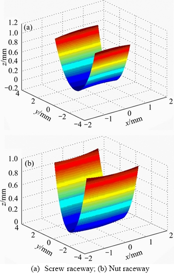
Figure 3 Geometrical shape of raceways:

The geometrical shape of two contact bodies can be described by two 2D arrays. The value of the 2D array presents the altitude value from the point to the project on the OXY system, and the value is determined by the altitude value of the adjacent point.

The points on the contact bodies appear in pairs. Two points of a pair are projected to the same point on the OXY system, therefore, the mesh of two bodies is the same on OXY. The region adjacent to the contact points is meshed, and the nodes are depicted by (i, j), where i is the column number and j is the row number.

The set of all nodes is given by:

           (10)

where M and N present the number of nodes in X and Y directions, respectively. The coordinates at node (i, j) are depicted by (x_i, y_j).

The sum of normal deformations of two contact surfaces at (x, y) is defined as u(x, y). It can be obtained by the normal contact stress p(x, y) [23], and the expression is given by:

       (11)

where K(x, y) is the affecting coefficient of normal deformation, which is the normal deformation at (x, y) when a unit normal force is subjected at the origin. The affecting coefficient of normal deformation K(x, y) can be expressed by the Boussinesq equation [23]:

                    (12)

where E is the elasticity modulus of the ball and raceway, and v is the Poisson ratio.

2.2.2 Normal contact stress analysis

The region is meshed into M×N elements, where (i, j) represents the center of element. The normal contact stress in every element is approximate to be constant, and the discrete form of Eq. (11) is given by:

,           (13)

where u_i,j is the normal deformation of nodes (i, j), and p_k,l is the normal stress subjected on the element with a center of (k, l).

K_i,j is the affecting coefficient, defined as:

,      (14)

where S₀ is the meshed region.

The contact problem of ball/raceway can be described as follows:

        (15)

       (16)

,                        (17)

                       (18)

                         (19)

where δ_z is the relative rigid displacement between balls and raceways; I_C is the set of all nodes in contact; d_s is the area of elements; F_z is the total normal load.

The normal contact stress p_i,j on the contact surface can be obtained by solving Eqs. (15)–(19). Generally, the contact region is undetermined before the contact problem is solved, and the relative rigid displacement δ_z is also undetermined. In Sections 2 and 3, only the initial preload is considered. Preload variation induced by axial load and its effect on thermal contact resistance are discussed in Section 4. The total normal load F_z can be calculated by the initial preload of ball screws according to the equilibrium equation of nuts. The expression can be given by:

                        (20)

where F_WS is the initial preload of ball screws, searchable in manufacturers’ catalogs; n_b is the number of balls in contact.

The contact problem is solved by the conjugate gradient method to expedite convergent speed of the iterative operation. During iteration, deformations in the contact region are calculated from the contact stress by fast Fourier transformation (FFT).

The 2D FFT is used to solve the elastic deformation problem between balls and raceways. Compared with other methods, the FFT is significantly effective [24]. Detailed steps of calculation are listed as follows:

1) The normal contact stress is expressed as the matrix P in M×N order. A matrix P′in 2M×2N order is assigned to P with the absent element replaced by zero.

2) The influence coefficient matrix K in the 2M×2N order is calculated.

3) A Fourier transformation is conducted for matrices P′ and K, respectively. and in the 2M×2N order are obtained.

4) The transformation matrixin the frequency domain can be obtained from the production of corresponding elements in and . The deformation matrix T can be obtained from the inverse Fourier transform of.

5) An assumption of is made. The deformation in the contact region u_i,j is obtained.

The contact problem described by Formulas (15)–(19) is a linear complementary problem that can be given by:

                          (21)

                (22)

where is the element of the constant matrix is the convolution symbol.

According to the variational principle in contact mechanics, the contact problem described by Eq. (21) is equivalent to the conditional extremum problem of quadratic function [25, 26], and it can be given by:

                    (23)

where represents the sum of products of corresponding elements in the two matrices; P is the stress distribution; U is the deformation distribution with the corresponding element u_i,j; H is the initial gap with the corresponding element h_i,j, which can be obtained by geometrical shape of the raceways in Section 2.1.

The conjugate gradient method is used for the contact problem solution. The flowchart is depicted in Figure 4, and detailed steps of calculation are listed as follows [27]:

1) The initial normal stress P for the iterative process should be given and the element of P should be non-negative p_i,j≥0. Equation (19) should be also satisfied in the meshed region. The solution coefficient in the conjugate direction is assigned λ=0, G_old=0. The iteration precision ε₀ should be assigned before the iterative process starts.

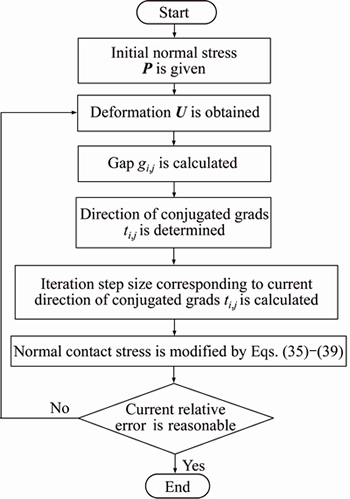
Figure 4 Flowchart of normal contact stress analysis

2) The deformation U, satisfying Eq. (13), is calculated by the FFT in every iterative process. The detail steps of calculation are listed above.

3) The gap g_i,j is calculated in the meshed region, and the gap average is adjusted.

                (24)

                        (25)

                  (26)

where N_c is the number of nodes in the contact region I_c; I_c is the current contact region, where all nodes satisfy the p_i,j≥0 condition.

4) The direction of conjugated grads t_i,j is determined. The quadratic sums of gaps in the contact region are calculated firstly.

                           (27)

The new directions of conjugated grads t_i,j are calculated:

          (28)

                        (29)

The newly obtained t_i,j is the deepest descent direction. The current value G is saved for the next iteration G_old=G.

5) In order to calculate the iteration step size corresponding to current direction of conjugated grads t_i,j, the convolution of affecting coefficient K_i,j and the direction of conjugated grads t_i,j are calculated by the FFT.

            (30)

The average of r_i,j is adjusted.

                         (31)

                   (32)

The iteration step size τ corresponding to the current direction of the conjugated grads t_i,j is determined by:

                         (33)

6) The normal contact stress is modified. The stress distribution is saved for error evaluation.

                     (34)

Consequently, the normal stress distribution is updated according to the direction of the conjugated grad t_i,j and step size τ.

                (35)

7) All stress values being negative are replaced by 0, whereas, the corresponding nodes are assigned to be overlapped but not on the contact status.

         (36)

8) If λ is replaced by 1; otherwise, it is replaced by 0. Consequently, the normal stress of overlapped nodes is updated as follows:

               (37)

It can be observed that τ>0 is always satisfied, therefore, all overlapped nodes turn into contact regions following update by Eq. (36).

9) The current normal load is calculated, therefore, the equilibrium equation should be satisfied:

                         (38)

              (39)

10) The current relative error is evaluated by:

                 (40)

If ε≥ε₀, the iterative process continues from Steps (2)–(10); otherwise, it ends.

The normal stress on the contact surface in the ball screw is solved by this method, as presented in Figure 5. From Figure 5, it is concluded that normal contact stress distribution of screw-raceway/ball and nut-raceway/ball contacts is similar. The contact stress of nut-raceway/ball is smaller than that of screw-raceway/ball. The reason is that the screw-raceway in the tangent direction is convex, while the nut-raceway in the tangent direction is concave. The contact region can also be predicted by Figure 5.

2.3 Thermal contact resistance

Regarding contact stress as obtained in Section 2.2, thermal contact resistance of every diminutive area is solved by the MB fractal theory. The micro-topography of contact surfaces can be considered in the MB fractal theory compared with other methods.

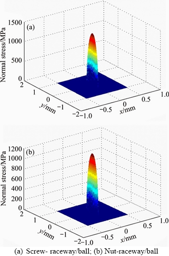
Figure 5 Normal contact stress distribution:

Contact between two contact surfaces occurs only at certain discrete diminutive areas due to actual rough surfaces. The asperity on rough surfaces can be simplified to a sphere [28]. The contact area of asperities a_c at the critical status of elastic and plastic deformation is given by:

                        (41)

where H is the lower hardness

of two contact materials; σ_y is the lower yield strength of the two materials; G is the scale parameter of the contact surface; D is the fractal dimension of the surface profile. It describes irregular patterns of the surface profile in all scales.

The relationship between deformation of asperities δ and the corresponding critical value δ_c can be expressed by:

 (1

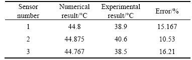
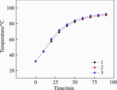
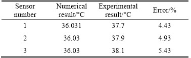
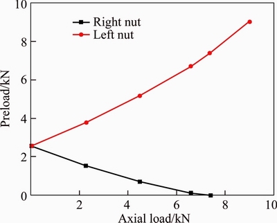
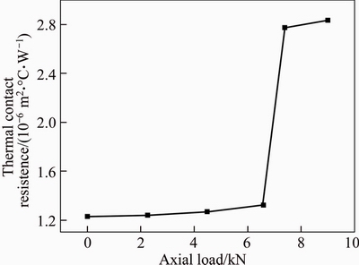
where a is the contact area of the asperity. If ac, according to Eq. (42), then δ_c<δ and plastic deformation occurs on the asperity. If a>a_c, the δ_c>δ can be obtained, where elastic deformation occurs on the asperity.

According to the MB fractal theory, thermal contact resistance of the diminutive area is given by [29, 30]:

         (43)

where λ₁ and λ₂ are the thermal conductivities of materials of the ball and nut/screw; λ_f is the thermal conductivity of the medium between them; A is the apparent contact area in the diminutive area, defined in Section 2.2; L_g is the thickness of space between the ball and nut/screw, expressed as [11]:

            (44)

where z is the height of the asperity; L_u is the fractal domain length; a_l is the maximum of the contact area at the contact points. a_l can be solved by Eq. (45).

   (45)

where P is the normal load on the diminutive area, equal to p_i,jA.

ψ is the domain extension factor, obtained by solving Eq. (46):

            (46)

is the real-apparent contact ratio, given by:

 (47)

Since the thermal contact resistance of every diminutive area is obtained, the total thermal contact resistance at the contact region is given by:

                          (48)

For a screw-ball-nut contact, the thermal contact resistance can be expressed as:

                          (49)

where R_sb is the thermal contact resistance at the screw-ball contact region and R_bn is the thermal contact resistance at the nut-ball contact region.

Regarding the ball screws, the thermal contact resistance is determined by:

                           (50)

where R is the total thermal contact resistance of the ball screw; R_sbn,k is the thermal contact resistance at the k-th screw-ball-nut contact region.

3 Validation

In order to validate the modeling approach for thermal contact resistance of ball screws, a self- designed experiment is implemented.

3.1 Experimental setup

It is difficult to validate this modeling approach in actual working condition. Therefore, a fundamental experiment is conducted to validate the approach. The experimental setup in this research is depicted in Figure 6. In this experiment, the nut and screw are static, and no axial load is applied. The initial preload of ball screws can be searched in manufacturers’ catalogs. This experiment is carried out at room temperature. The temperature is retained constant during the experiment. In order to avoid heat exchange between the specimen and the external environment, the specimen is wrapped around an asbestos cloth during the experiment, as presented in Figure 7. The high-temperature ceramic heating sheet (XH-RJ101012 type) is attached onto the inner lining of the nut through magnetic adsorption. The heat flows from the inner lining of the nut to the screw through the nut-ball-screw contact region. The heating sheet is powered by a DC stabilized power supply (HY1711D₂-5S type). The supply voltage is 24 V. Two ultra-thin temperature sensors (KYW-TC type) are arranged. One is attached onto the inner lining of the nut, whereas the other is attached to the screw, as presented in Figure 8. A temperature-circuit-detect instrument is employed for temperature tracking.

Figure 6 Experimental setup

Figure 7 Asbestos cloth wrapping around specimen

Figure 8 Sensor and heating sheet location

The temperature is tracked during the experiment, as presented in Figure 9. The temperature increases in the experimental time duration, reaching a balance following a 1.5-h period. Similar experiments are conducted when the supply voltage is 12 V and 6 V.

3.2 Analysis and comparisons

In the finite element software, the thermal contact resistance in unit area is usually required.

Figure 9 Temperature variation

Therefore, the thermal contact resistance in a unit area is analyzed in this section.

Thermal contact resistance in a unit area can be described by the ratio of temperature variance between two contact surfaces to the average heat flux, crossing the contact surfaces.

                        (51)

where T₁ and T₂ are the temperatures of the two contact surfaces, respectively. These temperatures could not be measured directly during the experiment, therefore they are determined by measuring the temperature of nodes being near the contact surfaces. S is the apparent contact area, as described in Section 2. Q is the heating power, determined by Q=U²/R, where U is the supply voltage of the DC stabilized power supply, and R is the resistance of the heating sheet, which could be measured by an ohmmeter. According to the temperature value measured in Section 3.1, the experimental value can be determined as shown in Table 2.

Table 2 Comparison between results of thermal contact resistamoes

The machining technology of balls is more mature compared with that of raceways. Therefore, the micro-topography of ball surfaces is neglected. The surface topography of raceway is measured, depicted in Figure 10. The average of fractal parameters is obtained. D=1.59, G=9×10^–10. The fractal parameter is introduced to the fractal theory. According to Section 2, the theoretical value could be determined as shown in Table 2. Through comparison, the result obtained by the analytical method in this research agrees well with the experimental result. The maximum error between theoretical and experimental results at different conditions is 14%.

Figure 10 Measurement of surface topography

The comparison between theoretical and experimental results demonstrates that the analytical method combining the minimum excess principle with the MB fractal theory could be implemented for thermal contact resistance estimation of ball screws. Compared with other methods, micro-topography of contact surfaces can be considered in the analytical method proposed in this research.

4 Discussion

4.1 Effects of fractal parameters

To investigate the effects of fractal parameters on thermal contact resistance of ball screws, various fractal parameters are introduced to the model. The discussion is conducted under the condition that only the initial preload is considered. Under the condition that the parameter G is fixed (G=0.138 nm), the thermal contact resistance decreases along with the increase of D, as presented in Figure 11(a). The reason is that the greater fractal dimension D of the contact surface would lead to the lower surface roughness [31], whereas a significantly smoother surface would result in a further lower thermal contact resistance.

Similar investigation is conducted under the condition that the parameter D is fixed (D=1.475), and thermal contact resistance increases along with an increase in G, as presented in Figure 11(b). The reason is that the greater scale parameter G of the contact surface would lead to the higher fluctuations of surface profile curves, resulting in a significantly rougher surface. The rougher surface would generate a greater thermal contact resistance.

Figure 11 Effects of fractal parameters on thermal contact resistance:

4.2 Effects of axial load

Under the actual working condition, the nut is mainly subjected to axial load. For fixed-position pretension ball screws, the axial load would lead to the preload of one nut increasing, whereas the preload of the other nut decreases according to the axial deformation consistency of the two nuts under the preload status, presented in Figure 12. The contact status of left nut and that of right one are different. Thermal contact resistance of ball screws would vary due to the variation of preload.

If the axial load is applied in the direction depicted in Figure 12, the preload of right nut will be zero when the axial load is over 3 times the initial preload [32]. While the axial load is applied in the opposite direction, which is towards right. The preload of left nut will be negative when the axial load is over 3 times the initial preload [33]. The first situation which is depicted in Figure 12 is discussed in this research.

Figure 12 Sketch of nuts subjected to axial load

In our former studies [32], the relationship between the axial load and preload of the two nuts is investigated. According to the method in our former studies, the preload of the two nuts can be obtained along with axial load increase, as presented in Figure 13.

Based on the preload of the two nuts depicted in Figure 13, the thermal contact resistance of the ball screws can be determined according to the series or parallel connections among them, as presented in Figure 14. The conclusion could be drawn that thermal contact resistance of ball screws is retained almost constant along with axial load increase before the preload of the right nut turns into zero. When the axial load reaches 3 times the initial preload, the right nut loses touch with the screw, and the preload of the right nut turns into zero [32]. The thermal contact resistance of ball screws grows when the preload of right nut turns into zero. The reason is that the ball screw turns into a single-nut ball screw in this situation, whereas the heat exchange occurs only on the left nut, leading to a greater thermal contact resistance.

5 Application

The aim of thermal contact resistance modeling is to predict the temperature distribution accurately in ball screws. A finite element model of ball screws is established with the thermal contact resistance determined by the proposed method in Section 2. The temperature distribution of a certain ball screw is predicted. The temperature of nuts is measured in a self-designed test bed to validate the finite element model of ball screws.

Figure 13 Preload of two nuts

Figure 14 Thermal contact resistance considering axial load

As shown in Figure 15, the finite element model includes the nuts, the screw shaft, the balls and the spacer. Because of the asymmetry caused by lead angle in ball screws, a 3D model is established. The nut remains static in the middle of the screw shaft during the simulation [34]. In order to increase calculation efficiency, the screw shaft section which is not in contact status with balls is simplified by neglecting the thread.

The heat flow from the bearing is determined as

                             (52)

where Q_be is the heat flow from the bearing; M_be is the frictional torque, which is provided in manufacturers’ catalogs; ω is the rotation speed. Half of the heat flow is applied in the corresponding end of the ball screw.

The heat flow from the ball screw interface is determined as

Figure 15 Finite element model of ball screws:

                             (53)

where Q_be is the heat flow from the ball screw interface; M_be is the drag torque of ball screw. Drag torque of ball screw can be determined by force analysis on balls, which will be presented in another paper. The heat flow is applied at the ball-nut and ball-screw contact point. The thermal contact resistance is calculated by this proposed method and applied at the ball-nut and ball-screw contact.

The convention coefficient depends on the solid shape and speed. A detail method for determining the convention coefficient is presented in Ref. [35]. The modeling approach for thermal contact resistance in Section 2 is introduced to the finite element model. The finite element model contains 95502 elements and 167410 nodes.

The temperature of nuts is measured in a self-designed test bed to validate the finite element model, which is depicted in Figure 16 (a). The test bed consists of a table moved by a double-nut ball screw with three temperature sensors attached on it. Three sensors are mounted on the nut, which is shown in Figure 16(b). The motor rotates at the speed of 1000 r/min until the temperature is balanced. There is no axial load applied on the nut. Only initial preload is considered. The value of temperature sensors is tracked, as presented in Figure 17. The temperature increases during the experiment, reaching a balance following a 1.5 h period. The temperature rising trend agrees with the former research [36].

Figure 16 Experimental setup:

The comparison between experimental results and theoretical ones is conducted, which is shown in Table 3. It is concluded that the result obtained by the finite element model agrees well with the experimental result. The maximum error at different positions is 16.21%. The error is acceptable in engineering practices.

Similar finite element analysis on the condition that the screw speed is 800 r/min is also conducted. The corresponding experiment on this condition is also carried out. The temperature rise of nut is depicted in Figure 18. The temperature trend is similar with that of screw speed 1000 r/min. The comparison between the results obtained by the two methods shown in Table 4 reveals that the maximum error at different positions is 5.43%. The error is also acceptable in engineering practices. The comparisons in different conditions indicate the approach for thermal contact resistance in ball screws could be applied in finite element model to predict the temperature distribution.

Figure 17 Temperature variation during experiment with screw speed of 1000 r/min

Table 3 Comparison between numerical results and experimental results of temperature with screw speed of 1000 r/min

Figure 18 Temperature variation during experiment with screw speed of 800 r/min

Table 4 Comparison between numerical results and experimental results of temperature with screw speed of 800 r/min

6 Conclusions

The following conclusions can be drawn from modeling of the thermal contact resistance of ball screws.

1) A new analytical method combining the minimum excess principle with the MB fractal theory is proposed for thermal contact resistance of ball screws estimation in this research. The minimum excess principle is employed to conduct normal stress analysis. The MB fractal theory is adopted to obtain contact stiffness in ball screws. Microscopic fractal characteristics of the interfaces could be considered in this method.

2) The effectiveness of the proposed method is validated by the self-designed experiment. The comparison between theoretical and experimental results demonstrates that thermal contact resistance of ball screws can be obtained by the method.

3) Effects of fractal parameters on thermal contact resistance of ball screws are discussed in this research. Under the same scale parameters, thermal contact resistance decreases along with fractal dimension increase. Under the same fractal dimension, thermal contact resistance increases along with the increase of scale parameter. Effects of the axial load on thermal contact resistance of ball screws are also investigated. Thermal contact resistance of ball screws is retained almost constant along with axial load increase before the preload of the right nut turns into zero, and the thermal contact resistance of ball screws grows when the preload of right nut turns into zero.

4) An application of the proposed method in real ball screw is conducted. A finite element model of ball screws is established with the thermal contact resistance determined by the proposed method. The temperature distribution of a certain ball screw is predicted and compared with experimental results. The comparison indicates the approach for thermal contact resistance in ball screws could be applied in finite element model to predict the temperature distribution.

Appendix I

Notation

a

Area/mm²

h

Initial gap/mm

n

Number

p

Normal stress of element/Pa

r

Radius/mm

u

Displacement of element/mm

x, y, z

Coordinates in AX_AY_AZ_A or BX_BY_BZ_B

E

Elasticity modulus/MPa

F

Force/N

G

Scale parameter of the contact surface/μm

H

Lower hardness of two contact materials/ MPa

K

Affecting coefficient of normal deformation/(mm·N^–1)

L

Lead/mm

M, N

Total number in the X or Y direction

P

Load/N

Q

Heating power/W

R

Thermal contact resistance/(°C·m²·W^–1)

S

Apparent contact area/mm²

U

Supply voltage/V

α

Lead angle/(°)

β

Thread angle/(°)

δ

Displacement/mm

ε

Iteration precision

θ

Coordinate transformation angle/(°)

λ

Thermal conductivities/(W·°C·m^–1)

v

Poisson ratio

Σ

Lower yield strength of the two materials/ MPa

τ

Iteration step size

ψ

Domain extension factor

ω

Rotation speed/(r·min^–1)

Subscripts and superscripts

1, 2

The two contact surfaces

b

Ball

be

Bearing

bn

Ball-nut

bs

Ball screw

c

In contact status or critical

f

Medium

g

Gap

i, j

Column or row number

k

A or B

k, l

Element number

l

Maximum

r

Real-apparent contact ratio

s

Screw

sb

Screw-ball

sbn

Screw-ball-nut

A     

Contact point between ball and screw raceway

AS    

Arc in the cross section of the screw-raceway

B    

Contact point between the ball and nut raceway

BS    

Arc in the cross section of the nut-raceway

N     

Nut

WS   

Preload of ball screw

References

[1] ZHANG Hui-jie, ZHANG Jun, LIU Hui, LIANG Tao, ZHAO Wan-hua. Dynamic modeling and analysis of the high-speedballscrewfeed system [J]. Proceedings of the Institution of Mechanical Engineers, Part B: Journal of Engineering Manufacture, 2015, 229(5): 870–877.

[2] ZHANG Jun,LI Bo,ZHOU Chang-xing,ZHAO Wan-hua. Positioning error prediction and compensation ofballscrewfeed drive system with different mounting conditions [J]. Proceedings of the Institution of Mechanical Engineers, Part B: Journal of Engineering Manufacture, 2016, 230(12): 2307–2311.

[3] ATTIA M H, KOPS L. On the role of fixed joints in thermal deformation of machine tool structures [J]. Annals of the CIRP , 1978, 27(1): 305–310.

[4] LI Fu-ping, LI Ying, LIU Zhi-feng, HU Qiu-shi, LIU Jian-yong, LI Yan. Thermodynamic performance analysis and improvement for cross-saddle type slide of electric discharge machine [J]. Vibroengineering Procedia, 2015, 5: 9–14.

[5] MIN X, JIANG S. A thermal model of a ball screw feed drive system for a machine tool [J]. Proceedings of the Institution of Mechanical Engineers, Part C: Journal of Mechanical Engineering Science, 2011, 225(1): 186–193.

[6] BOSSMANNS B, TU J F. A thermal model for high speed motorized spindles [J]. International Journal of Machine Tools & Manufacture, 1999, 39(9): 1345–1366.

[7] JIN Chao, WU Bo, HU You-min, YI Peng-xing, CHENG Yao. Thermal characteristics of a CNC feed system under varying operating conditions [J]. Precision Engineering, 2015, 42(4): 151–164.

[8] JIANG S, ZHENG Y. An analytical model of thermal contact resistance based on the Weierstrass-Mandelbrot fractal function [J]. Proceedings of the Institution of Mechanical Engineers, Part C: Journal of Mechanical Engineering Science, 2010, 224(4): 959–967.

[9] XU Rui-ping, XU Lie, ZHAO Lan-ping. Fractal description of thermal contact resistance between rough surfaces [J]. Journal of Shanghai Jiao Tong University, 2004, 38(10): 1609–1612. (in Chinese)

[10] ZOU Ming-qing, YU Bo-ming, CAI Jian-chao, XU Peng. Fractal model for thermal contact conductance [J]. Journal of Heat Transfer, 2008, 130(10): 101301.

[11] LIU Zhi-feng, PAN Ming-hui, ZHANG Ai-ping, ZHAO Yong-sheng, YANG Yong, MA Cheng-yu. Thermal characteristic analysis of high-speed motorized spindle system based on thermal contact resistance and thermal- conduction resistance [J]. International Journal of Advanced Manufacturing Technology, 2015, 76(9–12): 1913–1926.

[12] CUI Ling-li, HUANG Jin-feng, ZHANG Fei-bin. Quantitative and localization diagnosis of a defective ball bearing based on vertical-horizontal synchronization signal analysis [J]. IEEE Transactions on Industrial Electronics, 2017, 64(11): 8695–8705.

[13] WEN Shu-tao, TAN Yi, SHI Shuang, DONG Wei, JIANG Da-chuan, LIAO Jiao, ZHU Zhi. Thermal contact resistance between the surfaces of silicon and copper crucible during electron beam melting [J]. International Journal of Thermal Sciences, 2013, 74(6): 37–43.

[14] SALGON J, ROBBE-VALLOIRE F, BLOUET J, BRANSIER J. A mechanical and geometrical approach to thermal contact resistance [J]. International Journal of Heat and Mass Transfer, 1997, 40(5): 1121–1129.

[15] SADEGHIFAR H, DJILALI N, BAHRAMI M. A new model for thermal contact resistance between fuel cell gas diffusion layers and bipolar plates [J]. Journal of Power Sources, 2014, 266: 51–59.

[16] SADEGHIFAR H, DJILALI N, BAHRAMI M. Counter-intuitive reduction of thermal contact resistance with porosity: A case study of polymer electrolyte membrane fuel cells [J]. International Journal of Hydrogen Energy, 2016, 41(16): 6833–6841.

[17] TANG Qing-yun, ZHANG Wei-fang. The effect of pressure on thermal contact conductance of superalloys under high temperature [J]. International Journal of Heat and Mass Transfer, 2016, 103: 1208–1213.

[18] MO Jing-wen, BAN Heng. Measurements and theoretical modeling of effective thermal conductivity of particle beds under compression in air and vacuum [J]. Case Studies in Thermal Engineering, 2017, 10: 423–433.

[19] ZHANG Guo-dong, ALBERDI R, KHANDELWAL K. Analysis of three-dimensional curved beams using isogeometric approach [J]. Engineering Structures, 2016, 117(15): 560–574.

[20] CHERN S S, CHEN W H, LAM K S. Lectures on differential geometry [M]. Singapore: World Scientific, 2000.

[21] CONDE B, DROSOPOULOS G A, STAVROULAKIS G E, RIVEIRO B, STAVROULAKI M E. Inverse analysis of masonry arch bridges for damaged condition investigation: Application on Kakodiki bridge [J]. Engineering Structures, 2016, 127(15): 388–401.

[22] POLONSKY I A, KEER L M. A numerical method for solving rough contact problems based on multi-level multi-summation and conjugate gradient techniques [J]. Wear, 1999, 231(2): 206–219.

[23] JOHNSON K L. Contact mechanics [M]. London: Cambridge University Press, 1985.

[24] LIU Shuang-biao, WANG Qian. Study contact stress fields caused by surface tractions with a discrete convolution and fast Fourier transform algorithm [J]. ASME Journal of Tribology, 2002, 124(1): 36–45.

[25] TIAN Xue-feng, BHUSHAN B. A numerical three- dimensional model for the contact of rough surfaces by variational principle [J]. ASME Journal of Tribology, 1996, 118(1): 33–42.

[26] STANLEY H M, KATO T. An FFT-based method for rough surface contact [J]. ASME Journal of Tribology, 1997, 119(3): 481–485.

[27] NOCEDAL J, WIGHT S. Numerical optimization [M]. Beijing: Science Press, 2006.

[28] ZHANG Xue-liang, HUANG Yu-mei, HAN Ying. Fractal model of the normal contact stiffness of machine joint surfaces based on the fractal contact theory [J]. China Mechanical Engineering, 2000, 11(7): 727–729. (in Chinese)

[29] WANG S, KOMVOPOULOS K. A fractal theory of the interfacial temperature distribution in the slow sliding regime: part II—multiple domains, elastoplastic contacts and applications [J]. ASME Journal of Tribology, 1994, 116(4): 824–832.

[30] MAJUMDAR A, BHUSHAN B. Fractal model of elastic– plastic contact between rough surfaces [J]. ASME Journal of Tribology, 1991, 113(1): 1–11.

[31] GE Shi-rong, ZHU Hua. Fractal theory in tribology [M]. Beijing: China Machine Press, 2005. (in Chinese)

[32] HU Jian-zhong. Study on the accuracy degradation mechanism of the ball screw mechanism [D]. Beijing: Beijing University of Technology, 2014. (in Chinese)

[33] WEI Chung-chin, LIN Jen-fin, HORNG Jeng-haur. Analysis of a ball screw with a preload and lubrication [J]. Tribology International, 2009, 42(11, 12): 1816–1831.

[34] OYANGUREN A, LARRANAGA J, ULACIA I. Thermo- mechanical modelling of ball screw preload force variation in different working conditions [J]. The International Journal of Advanced Manufacturing Technology, 2018, 97(1–4): 723–739.

[35] GAO Xiang-sheng. Research on dynamic and thermal characteristics of high-speed machining centers and their key components [D]. Beijing: Beihang University, 2013. (in Chinese)

[36] SHI Hu, ZHANG Dong-sheng, YANG Jun, MA Chi, MEI Xue-song, GONG Guo-fang. Experiment-based thermal error modeling method for dual ball screw feed system of precision machine tool [J]. The International Journal of Advanced Manufacturing Technology, 2016, 82(9–12): 1693–1705.

(Edited by HE Yun-bin)

中文导读

滚珠丝杠副接触热阻的建模与应用

摘要：为了求解滚珠丝杠副的接触热阻，提出了一种基于最小余能原理和MB分形理论的解析方法。该方法在求解接触热阻时可考虑接触面的微观分形特征。采用最小余能原理求解法向应力分布，进而采用MB分形理论求解接触热阻。通过自行设计实验验证了该方法的有效性。理论和实验的结果对比说明，该方法可准确获得滚珠丝杠副接触热阻。在此基础上，讨论了分形参数对滚珠丝杠副接触热阻的影响，分析了螺母轴向载荷对滚珠丝杠副的接触热阻的影响。结果表明，接触热阻随着分形参数D的增加而减小，随着尺度参数G的增加而增加。在右螺母预紧力变为零之前，滚珠丝杠副接触热阻随着轴向载荷的增加几乎保持不变。最后，开展了该建模方法在自行设计试验台的应用，开展了相应的温度测试，进一步验证了该方法的有效性。

关键词：滚珠丝杠副；分形理论；接触热阻；接触应力；预紧力

Foundation item: Projects(51875008, 51505012, 51575014) supported by the National Natural Science Foundation of China; Project supported by the China Scholarship Council

Received date: 2017-10-11; Accepted date: 2018-09-25

Corresponding author: GAO Xiang-sheng, PhD, Associate Professor; Tel: +86-10-67392137; E-mail: gaoxsh@bjut.edu.cn; ORCID: 0000-0001-5947-5826