J. Cent. South Univ. Technol. (2008) 15(s1): 316-321

DOI: 10.1007/s11771-008-371-6

Prediction of shear bands in sand based on granular flow model and two-phase equilibrium

ZHANG Yi-tong(张义同)¹, QI De-xuan(齐德瑄)¹, DU Ru-xu(杜如虚)², REN Shu-guang(任述光)³

(1. Department of Mechanics, School of Mechanical Engineering, Tianjin University, Tianjin 300072, China;

2. Shenzhen Institute of Advanced Technology, Chinese Academy of Sciences, Shenzhen 518067, China;

3. College of Engineering and Technology, Hunan Agricultural University, Changsha 410128, China)

Abstract: In contrast to the traditional interpretation of shear bands in sand as a bifurcation problem in continuum mechanics, shear bands in sand are considered as high-strain phase (plastic phase) of sand and the materials outside the bands are still in low-strain phase (elastic phase), namely, the two phases of sand can coexist under certain condition. As a one-dimensional example, the results show that, for materials with strain-softening behavior, the two-phase solution is a stable branch of solutions, but the method to find two-phase solutions is very different from the one for bifurcation analysis. The theory of multi-phase equilibrium and the slow plastic flow model are applied to predict the formation and patterns of shear bands in sand specimens, discontinuity of deformation gradient and stress across interfaces between shear bands and other regions is considered, the continuity of displacements and traction across interfaces is imposed, and the Maxwell relation is satisfied. The governing equations are deduced. The critical stress for the formation of a shear band, both the stresses and strains inside the band and outside the band, and the inclination angle of the band can all be predicted. The predicted results are consistent with experimental measurements.

Key words: strain localization; locally-deformed bands; shear bands; two-phase equilibrium; granular model of sand

1 Introduction

Strain localization has been observed for a long time both at the scale of geotechnical structures and in laboratory experiments, and the strain localization in sand has received particular attention^[1-6].

Of the above work, many researchers devoted their studies to experimental investigations, in particular, to design plane strain devices, attempted to analyze and describe the occurrence and patterns of locally-deformed bands, termed usually shear bands. In the meantime, a large amount of theoretical research has also been carried out, and the formation of shear bands is generally interpreted as a bifurcation problem in continuum mechanics^[7].

In this paper, we would like to provide another mechanism of strain localization in sand. Shear bands in sand are considered as a high-strain phase of sand, and the materials outside the bands are still in low-strain phase, namely, two phases of sand can coexist under certain condition. Two-phase equilibrium can appear in materials with strain-softening behavior^[8-9], and many experiments have revealed that sand with shear bands shows strain-softening behavior, see, e.g., the stress- strain curves in Ref.[4]. It can also be shown that the two-phase solution is stable compared with single-phase solutions^[10]. So that, from the viewpoint of bifurcation, it may therefore be argued that the two-phase solution is a stable branch of solutions. However, the method to find the two-phase solution is very different from the one for bifurcation analysis. For the analysis of two-phase equilibrium the discontinuity of deformation gradient and stress across interfaces between phases should be considered, and the continuity of displacements and traction and the Maxwell relation across interfaces must be imposed.

The slow plastic flow model^[11-12], which is more suitable for sand, is applied for the analysis of strain localization in sand.

2 Geometry of sand specimen

A top view of a sand specimen under plane strain is depicted in Fig.1. Locally-deformed band was signified by “+” phase, and the regions outside the locally-deformed band by “” phase, respectively. The N=[N₁, N₂, N₃]^T in Fig.1 is the unit vector normal to the interface between the “+” phase and a ‘’ phase in the reference configuration and points from the ‘+’ phase into the ‘’ phase.

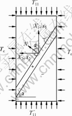
Fig.1 A top view of sand specimen under plane strain state

A common Cartesian coordinate system for both reference and deformed configurations is used in the present work. A typical material particle of the specimen, whose position vector in the reference configuration is denoted by (X₁, X₂, X₃), is assumed to have a position vector (x₁, x₂, x₃) in the deformed configuration. The X₁(x₁)-axis is along the compression direction as shown in Fig.1 and the X₃(x₃)-axis is along the thickness direction of the specimen. The deformation gradient tensor is defined by.

The inclination angle of the shear band to the compression direction, denoted by α as shown in Fig.1, is given by

α=arctan^-1(N₂/N₁)                    (1)                                         

3 Multi-phase equilibrium

Multi-phase equilibrium requires that the following equilibrium equations away from interfaces between phases must be satisfied (in the absence of body forces)

                                     (2)                                         

where  div is the divergence operator in the reference configuration, π is the first Piola-Kirchhoff stress tensor, and the superscript T signifies the transpose of tensors.

The stress across interfaces is generally discontinuous, i.e. in general  across interfaces, where the superscripts (sometimes subscripts) ‘+’ or ‘’ signify evaluation at an interface as it approaches the interface from the two sides, respectively. When there is no ‘’ or ‘+’ superscript/subscript attached to a field variable evaluated at an interface, it means that the variable can be evaluated on either side of the interface.

For continuum the continuity of traction across interfaces must be satisfied, namely

                                        (3)                                       

where  [g]=g⁺-g^- is defined as a jump of the function g across an interface.

For continuum, the continuity of displacements across interfaces must also be imposed. It means that the jump [F] must necessarily take the following form^[13]:

                                   (4)                                     

where  f is a vector and can be written as

                                         (5)                                    

In addition, the following Maxwell relation is also imposed as a necessary condition that ensures stability with respect to perturbations of the interface in the undeformed configuration^[13]:

,                               (6)                                  

where  W is the stress-work function that satisfies

 (7)                             

with T_AB and E_AB are the components of the second Piola-Kirchhoff stress tensor T and the Green strain tensor E, respectively.

For piecewise-homogenous deformations, the equilibrium equations are trivially satisfied, so multi- phase equilibrium can occur if only Eqns. and are satisfied.

4 A one-dimensional example of two-phase equilibrium

In order to explain some of the key ideas of two-phase equilibrium, a one-dimensional example of two-phase equilibrium was provided in this section briefly^[10].

A bar having uniform diameter was considered, occupying the region 0＜x＜L, and being composed of elastoplastic material with strain-softening behavior. The stress-strain curve for the material is shown in Fig.2.  For simplicity the Young modulus and the hardening modulus take the same value, denoted by μ. And it is supposed that the left boundary of the bar is fixed and the right boundary is subjected to a prescribed displacement δ in the x-direction.

It is easy to find the solutions for the bar.

Solution 1  For a given δ, when -1＜δ/L＜π_max/μ (i.e. -1＜γ＜γ_max) all the particles of the bar are in elastic phase, and a single-phase solution is obtained:

 (0＜x＜L)     (8)

where  γ(x), π(x) and u(x) are the strain, stress and

Fig.2 Stress—strain curve under uniaxial tension

displacement at x, respectively.

Solution 2  When   ＞ (i.e. γ＞γ_min), where  as shown in Fig.2, a single-phase solution (plastic solution) is obtained:

(0＜x＜L)(9)

Namely, when the prescribed elongation is sufficiently large every material particle is in the plastic phase.

Solution 3  When   ≤≤ (i.e.

γ_max≤γ≤γ_min), there is of course a solution with uniform strain associated with the declining branch of the stress-strain curve, but that solution is unstable. It is nature to consider the possibility of a mixture of the elastic and plastic phases.

Let x=s denote the location of phase boundary, and suppose that the material particles inside the region (0, s) belong to the plastic phase and the ones inside the region (s, L) belong to the elastic phase. For one-dimensional problems the jump condition reduces to π⁺=π^-, i.e. the stress is constant throughout the bar, and the Maxwell relation can be described geometrically the constant stress, termed the Maxwell stress and labeled π_M, cuts off equal areas of the stress-strain curve (see Fig.2). And the strains inside the two phases are determined by making use of the relevant stress-strain relation, respectively. The two-phase solution can be found as follows:

             (10)

                       (11)

By Eqn.(11), as s=0, there is ; as s=L, there is . Thus, when

≤≤                                                      (12)

the two-phase solution exists. It is worth noting that the interval  is included in the interval , as shown in Fig.2.

Thus if the elongation δ/L lies in the interval (-1, the problem now has a unique solution. However, for each   there are two solutions, i.e., Solution-1 and the Solution-3; and associated with each   there are two solutions, i.e., Solution-2 and the Solution-3. In order to determine which one of the two solutions is stable, their energies were compared. Evaluating the energy   at each of the three solutions leads to the corresponding energies

                 (13)

  respectively. It can be readily verified that

                                       (14)

Therefore, whenever a two-phase solution and a single phase solution exist at the same value of δ, the two-phase solution has less energy. So the two-phase solution is stable.

The analysis of two-phase equilibrium for one- dimensional problems is simple, but it gives one significantly more insight into the mechanism of strain localization. The analysis of two-phase equilibrium under plane strain state is much more difficult and will be carried out in the following sections.

The slow plastic flow model for granular materials suggested the Coulomb yield criterion^[11]

                          (15)

where  n and s are co-ordinates normal and along the slip plane, the sign “-“ before σ_nn indicates that  the value of the compressive stress σ_nn should be negative, and the c and  are the cohesive strength and the friction angle, respectively.

Alternatively, the yield criterion can be expressed in the form of a yield function F, with the form^[14]

  (16)

where  I₁ is the first stress invariant, and J₂ is the second stress invariant of the deviatoric stress components. The θ is the Lode angle, which can be determined by

                     (17)

where  J₃ is the third stress invariant of the deviatoric stress components.

The incremental stress-strain relation can be expressed as

                                 (18)

where  L^ep is the fourth-order elastoplastic stiffness tensor, and for the loading case, there is

              (19)

with

         (20)

where  s_ij is the components of deviatory stress tensor, and C₁, C₂ and C₃ take the forms, respectively,

                                (21)

              (22)

                (23)

And the L_ABCD in Eqn.(19) are the components of the fourth-order elastic stiffness tensor L and are given by

                 (24)

where  G is the elastic shear modulus, δ_ij is the Kronecker delta, K is the bulk modulus, and  is the fourth-order special identity tensor with the following components

               (25)

The inverted form of L is the fourth-order elastic compliance tensor M and has the flowing form:

                         (26)

6 Analysis of strain localization in sand

6.1 Low-strain phase

The stress field inside the low-strain phase as shown in Fig.1, denoted by T^-, takes the form

                   (27)

where  v is the Poisson ratio and  is the confining pressure as shown in Fig.1. The corresponding strain, denoted by E^-, is given by

                                (28)

The deformation gradient can be assumed to be

                          (29)

and, from E=(F^TF-I)/2, the λ1 and λ₂ can be determined from

                (30)

The associated first Piola-Kirchhoff stress tensor is in the form

      (31)

and the strain energy is given by

                             (32)

6.2 High-strain phase

For the plane strain state, we can assume that

                            (33)

and that [F] takes the form of

                      (34)

From Eqn., we have

                             (35)

Then, for linearly hardening materials, we have consequently F⁺=F^-+[F],  and

                              (36)

Substituting Eqn.(36) into Eqn.(18) gives  and then there is

                               (37)

and

                            (38)

The stress-work function for plastic phase is given by For linearly elastic, linearly strain-softening and linearly hardening materials is

                  (39)

where   and  are the components of stress and strain at the upper yield point,  and  are the ones at the lower yield point, respectively.

6.3 Governing equations

Substituting Eqns.(33) and (38) into Eqn.(3) and substituting Eqns.(31)-(33), (36) and (39) into the Maxwell relation (6) give the following three equations

                     (40)

                    (41)

                      (42)

The two-phase piece-wise homogenous defor- mations can be in equilibrium only if Eqns.(40)-(42) together with  have a unique, real, physically acceptable solution for. The physically acceptability implies that for the specimen shown in Fig.1, where ＜0, N₁＞0 and N₂＞0, the real solution must satisfy f₁＜0 and f₂＞0 in order to ensure that [F₁₁]=f₁N₁＜0 and [F₂₂]=f₂N₂＞0, in other words, the material inside the locally-deformed band should be further compressed.

Eqns.(40)-(42) consist of polynomials for the variables N₁, N₂, f₁ and f₂, so they can be solved numerically by the polynomial homotopy continuation (PHC) algorithm. We discuss their numerical solutions in the following section.

7 Numerical solutions

As an illustration, the stress-strain curve of F3-sand in plane strain experiments given in Fig.9(b) in Ref.[4] is used to calibrate our model. From the curve, the values of the second Piola-Kirchhoff stresses, the Green strains, and the volumetric strains at the upper yield point and the lower yield point, and the elastic modulus can be evaluated as follows: =-112.5 kPa, -0.02, 0.015, -75 kPa, -0.04,  0.021, and E=5 625 kPa. And from Ref.[4] the friction angle and confining pressure take the value of φ=61.8? and T_c=-15 kPa. The Poisson ratio takes the value of 0.27 in the present analysis.

With the aid of PHC software package, numerically solving the calibrated Eqns.(40)-(42) together with  shows that

1) When ＞-90 there is no real solution for [N₁, N₂, f₁, f₂]^T.

2) When ＜-92 there are 8 real solutions for [N₁, N₂, f₁, f₂]^T. The 8 solutions can be divided into two groups. In each group the absolute values of the 4 solutions are the same to each other but their signs are different, i.e. in each group if  [N₁, N₂, f₁, f₂]^T is a solution, the [-N₁, N₂, -f₁, f₂]^T, [N₁, -N₂, f₁, -f₂]^T and   [-N₁, -N₂, -f₁, -f₂]^T are also the solutions. Namely, the number of the real solutions is always multiple of four.

3) The absolute values of the solutions in the two groups are different, but they are very close.

4) The 4 solutions in each group are in the forms of [N₁＞0, N₂＞0, f₁＜0, f₂＞0)^T, [N₁＜0, N₂＞0, f₁＞0, f₂＞0)^T, [N₁＞0, N₂＜0, f₁＜0, f₂＜0)^T  and [N₁＜0, N₂＜0,  f₁＞0, f₂＜0)^T respectively. The first one is a solution associated with the right-upward upper interface as plotted in Fig.1, the second one associated with the right-upward lower interface, and the third and fourth ones associated with the left-upward upper interface and left-upward lower interface, respectively. All the four solutions satisfy f₁N₁＜0 and f₂N₂＞0, so that they are all physically acceptable. Namely, both a left-upward shear band and a right-upward shear band in sand are possible as have been observed in experiments by many researchers, see, e.g., Fig.5 in Ref.[4]. Without loss of generality, in the following analysis only the solution  [N₁＞0, N₂＞0, f₁＜0, f₂＞0)^T is concerned.

5) -92+δ₁＜＜-91-δ₂ was chosen and it is found that when the values of δ₁ and δ₂ are greater and greater, the absolute values of the solutions in the two groups are closer and closer. Finally, we find that when

()_min=-91.310 9 (kPa)                      (43)

there is only a group of solutions in which the solution like [N₁＞0, N₂＞0, f₁＜0, f₂＞0)^T takes the following values:

         (44)

The stresses inside and outside the shear band are given, respectively, by

       (45)

          (46)

The strains inside and outside the shear band are given, respectively, by

        (47)

         (48)

From Eqn. we have

α=53.106 7?                                (49)

which agrees well with value of 57? measured by ALSHIBLI and STURE^[4] with error of 6.83%.

It is worth noting that no width of the locally-deformed band is concerned in the analysis above, so that the locally-deformed band with any width can occur in the specimen under the constant stress -91.310 9 kPa. In other words, it is theoretic- cally predicted that locally-deformed bands can spread while the specimen is compressed and the  keeps constant.

8 Conclusions

1) Based on the granular flow model of sand and the theory of two-phase equilibrium, the shear bands in sand are predicted successfully, the critical compressive stress, the inclination angle of the band, the stresses and strains both inside the band and the regions outside the band can all be predicted. Both left-upward shear bands and right-upward shear bands in specimens could happen theoretically.

2) It is worth noting that the discontinuity of displacement gradient and stress across interfaces between shear bands and other regions outside shear bands is considered in this work that is not considered usually in the bifurcation analysis.

References

[1] ROSCOE K H. The influence of strains in soil mechanics [J]. Geotechnique, 1970, 20(2): 129-170.

[2] ARTHUR J R F, DUNSTAN T, AL-ANI Q A J L, ASSADI A. Plastic deformation and failure in granular media [J]. Geotechnique, 1977, 27(1): 53-74.

[3] VARDOULAKIS I, GRAF B. Calibration of constitutive models for granular materials using data from biaxial experiments [J]. Geotechnique, 1985, 35(3): 299-317.

[4] ALSHIBLI K A, STURE S. Shear band formation in plane strain experiments of sand [J]. Journal of Geotechnical and Geoenvironmental Engineering, 2000, 126(6): 495-503.

[5] RECHENMACHER A L. Grain-scale processes governing shear band initiation and evolution in sands [J]. Journal of the Mechanics and Physics of Solids, 2006, 54: 22-45.

[6] DESRUES J, VIGGIANI G. Strain localization in sand: an overview of the experimental results obtained in Grenoble using stereophotogrammetry [J]. Int J Numer Anal Meth Geomech, 2004, 28: 279-321.

[7] VARDOULAKIS I, SULEM J. Bifurcation analysis in geomechanics [M]. London: Blackie Academic and Professional, 1995.

[8] ZHANG Y T, QIAO J L, AO T. Strain softening of materials and Lüders-type deformations [J]. Modeling and Simulation in Materials Science and Engineering, 2007, 15: 147-156.

[9] ZHANG Y T, REN S G, AO T. Elastoplastic modeling of materials supporting multiphase deformations [J]. Materials Science and Engineering A, 2007, 447: 332-340.

[10] ABEYARATNE R, BHATTACHARYA K, KNOWLES J K. Strain-energy functions with multiple local minima: Modeling phase transformations using finite thermoelasticity [C]// FU Y, OGDEN R W. Nonlinear Elasticity: Theory and Application. Cambridge: Cambridge University Press, 2001: 433-490.

[11] NEDDERMAN R M. Statics and kinematics of granular materials [M]. Cambridge: Cambridge University Press, 1992.

[12] JOP P, FORTERRE Y, POULIQUEN O. A constitutive law for dense granular flows [J]. Nature, 2006, 441: 727-730.

[13] FU Y B, FREIDIN A B. Characterization and stability of two-phase piecewise-homogeneous deformations [J]. Proc R Soc Lond A, 2004, 460: 3065-3094.

[14] ZIENKIEWICZ O C,PANDE G N. Some useful forms of isotropic yield surfaces for soil and rock mechanics [C]// GODEHUS G. Finite Elements in Gemechanics. New York: Wiley, 1977: 179-190.

(Edited by YANG You-ping)

Foundation item: Project(2007CB714001) supported by the National Basic Research Program of China (973 Program)

Received date: 2008-06-25; Accepted date: 2008-08-05

Corresponding author: ZHANG Yi-tong, Professor; Tel: +86-22-27404934; E-mail: ytzhang@tju.edu.cn