J. Cent. South Univ. Technol. (2011) 18: 618-626

DOI: 10.1007/s11771-011-0739-x

Optimal measurement configurations for kinematic calibration of six-DOF serial robot

LI Tian(黎田)¹, SUN Kui(孙奎)¹, XIE Zong-wu(谢宗武)¹, LIU Hong(刘宏)^{1, 2}

1. State Key Laboratory of Robotics and System, Harbin Institute of Technology, Harbin 150001, China;

2. Institute of Robotics and Mechatronics, German Aerospace Center, DLR, Germany

? Central South University Press and Springer-Verlag Berlin Heidelberg 2011

Abstract: An optimal measurement pose number searching method was designed to improve the pose selection method. Several optimal robot measurement configurations were added to an initial pre-selected optimal configuration set to establish a new configuration set for robot calibration one by one. The root mean squares (RMS) of the errors of each end-effector poses after being calibrated by these configuration sets were calculated. The optimal number of the configuration set corresponding to the least RMS of pose error was then obtained. Calibration based on those poses selected by this algorithm can get higher end-effector accuracy, meanwhile consumes less time. An optimal pose set including optimal 25 measurement configurations is found during the simulation. Tracking errors after calibration by using these poses are 1.54, 1.61 and 0.86 mm, and better than those before calibration which are 7.79, 7.62 and 8.29 mm, even better than those calibrated by the random method which are 2.22, 2.35 and 1.69 mm in directions X, Y and Z, respectively.

Key words: serial robot; pose selection; pose number; kinematic calibration; observability index

1 Introduction

Kinematic calibration is a process to improve absolute accuracy of robot manipulator by identifying inaccurate and unknown geometric parameters rather than changing the mechanical structure or design of the robot. It uses redundant measurements of joint variables and end-effector poses to identify the real values of the kinematic parameters and correct the robot kinematic model to improve the robot accuracy. There have been a lot of calibration methods since the beginning of 1980s. In general, most of these calibration processes are carried out in four steps: modeling, measurement, identification and correction [1].

Measurement of different poses of manipulator end-effectors is a crucial step in robot calibration procedure. Different measurement configurations contribute to end-effector errors variously. In some measurement configurations, the kinematic parameter errors of the robot do not influence end-effector pose errors much. In this situation, the noises associated with the measurement sensors become the main influence to the pose errors. Even though these noises sometimes are quite small, the influence on the end-effector accuracy is too large to ignore. To minimize the influence made by the sensors noises, robot measurement configurations in which the kinematic parameter errors cause the maximum end-effector errors should be selected. By differentiating the kinematic equation of manipulator, the direct proportion relationship between the kinematic parameter errors and the robot pose errors can be obtained. The relationship is expressed by the identification Jacobian matrix. As we know, the kinematic parameter errors are invariable. In order to get the maximum end-effector errors under invariable parameters, the measurement configurations that can maximize the identification Jacobian matrix should be selected. In other words, the measurement configurations that can best observe the kinematic parameter errors should be found. BORM and MENQ [2] proposed a concept named observability index to evaluate the observability of the identification Jacobian matrix for the kinematic parameter errors, or the goodness of measurement pose selection.

The observability indices always relate with the singular values of the identification Jacobian. Singular values of a matrix can be achieved by singular value deposition (SVD). Before the concept of observability indices, DRIELS and PATHRE proposed the condition number (termed its inverse as O_DP) which equals the ratio of the largest singular value to the smallest non-zero singular value [3]. The observability index proposed by BORM and MENQ is based on the product of all non-zero singular values of identification Jacobian matrix, which is termed as O_BM [4]. NAHVI et al [5] proposed the minimum singular value of identification Jacobian as an observability index, termed as O_NH1. NAHVI and HOLLERBACH [6] later proposed an observability index, the square of smallest non-zero singular value divided by the largest singular value of identification Jacobian, called the noise amplification index, here termed as O_NH2.

The current robot calibration algorithms [7-19] usually search for an optimal measurement configuration set using one of the four observability indices mentioned above as a criterion. ZHUANG et al [7] proposed a simulated annealing approach to obtain optimal or near optimal measurement configurations for robot calibration. To accelerate the convergence rate, a suitable cooling schedule was devised. The founding of a suitable cooling schedule was also the hard area of simulated annealing approach. The condition number and O_BM were used as the criteria of the pose selection process. In the later research, ZHUANG et al [8] adopted another optimal method, the genetic algorithm, to plan the robot calibration experiments. Condition number was selected as the criterion. DANEY et al [9] researched the influences of all these observability indices on calibration result of a Gough platform. Each observability index was used as a criterion to optimally select the robot poses, and the conclusion that the selected poses were localized at the boundary of the calibration workspace was obtained. Two kinds of multi-criteria optimization methods mixing two or more observability indices were proposed. One of the methods selected indices between O_BM and O_NH2 with a given probability alternatively, and the authors proved that it had poor improvement to calibration result. The other method used O_BM firstly to select poses as initial poses, and then picked up O_NH2 as a criterion to optimal 80% of initial poses. The latter gets better result. WATANABE et al [10] proposed an auto-calibration method for industry use based on vision measurement of camera. Calibration method for industry use should have such characteristics as low cost, time saving, and easy operation. The condition number was employed as an observability index to select the optimal set of poses. LIU and WANG [11] proposed the modified simulated annealing algorithm which used the observability index O_NH2 to select the optimal robot poses for five-DOF polishing robot. SUN and HOLLERBACH [12-13] proposed a new observability index (termed O_SH) based on the determinant of identification Jacobian to save time for searching the optimal pose set of a six-DOF PUMA 560 robot. In the aspect of pose choosing, an interesting algorithm named exchange-add-exchange algorithm to eliminate the unobservable poses was proposed. In addition, it was proved that the algorithm to maximize the determinant of identification Jacobian can select the same set of optimal poses with the algorithm maximizing O_BM. However, only the calibration result of kinematic parameters was given, and the improvement on the accuracy of end-effector was not mentioned. REN et al [14] proposed a new calibration method to improve the accuracy of parallel kinematics machine tools by keeping two attitude angles constant. A commercial biaxial inclinometer was installed on the end-effector to measure robot poses. The selected criterion of the optimal poses they adopted was the noise amplification index O_NH2.

The outcome proposed by these researchers is that the optimal robot poses localized at the boundary of the calibration workspace of parallel manipulator cannot be used on serial manipulators, because the rotation joints do not have actual motion boundary in their workspace, even worse, some boundary configurations of a serial robot are also their singular configurations. Meanwhile, the researches mentioned above do not consider the optimal number of measurement poses. It is well-known that the more the poses used in calibration, the higher the end-effector accuracy achieved. However, the pose errors of the end-effector cannot be infinitely decreased. Furthermore, the robot calibration is a time-consuming work. With the increase of measurement pose number, the time used in the identification of the geometric parameter will be dramatically prolonged. For this reason, an enough pose number which can obtain acceptable end-effector accuracy is needed. Recently, some researchers like VERL et al [20] and NATEGH and AGHELI [21] researched the optimal number of measurement pose problem, unfortunately both of their research objects were parallel manipulators.

In this work, a new optimal pose searching method is proposed, which includes an optimal measurement pose number seeking method in SUN’s exchange-add- exchange algorithm to search an optimal pose set for the calibration of a six-DOF serial lightweight manipulator (SLIMA).

2 Kinematic error model

The mechanical prototype of SLIMA is shown in Fig.1. It consists of six revolute mechatronic joints. The weightiest one of them is less than 1.2 kg. Modular concept is utilized in the last four joints to save research period and cost. The mechanical parts of every joint are designed with big central hole for passing most part of cables through inside of joints. After being passed through by control cables, there is no enough space for the cables of the end dexterous hand and camera. These cables can only be placed outside. To simplify the inverse kinematics, the last three joints are designed as a spherical wrist, which means the axes of last three joints intersect at one point O₄ or O₅, as shown from Fig.2.

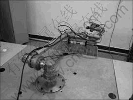
Fig.1 Six-DOF light-weight serial robot manipulator

The joints rotation direction, D-H frame assignment and kinematic model of the robot are shown in Fig.2. J_i (i=1, 2, 3, 4, 5, 6) represents axis of joint i. The first coordinate frame O₀-X₀Y₀Z₀ {O₀} is attached on a truss which is immobile to the ground. The last frame O₆-X₆Y₆Z₆ {O₆} is bound together with the end-effector whose centroid coincides with the origin O₆. Z₆ is set to be parallel to the last joint axis Z₅ to make kinematic modeling simple. X₀ is collinear with X₁ for the same reason. In the configuration in Fig.2, X₀, X₁, X₂, Z₃, Y₄, Z₅ and Z₆ are also coaxial.

After the assignment of the coordinate frames of every joint, D-H kinematic parameters and joint rotation range can be indicated, as listed in Table 1. β_i in Table 1 is the rotation angle of frame O_i-X_iY_iZ_i with respect to axle Y_i. It was firstly proposed by HAYATI to handle the kinematic error modeling problem of those robots that had two parallel consecutive axes. It is worth mentioning that the errors of kinematic parameter d_i would become significant when an error makes two axes Z_i-1 and Z_i not rigorously parallel. HAYATI proposed a new kinematic parameter error, Δβ_i, to substitute Δd_i to donate this inaccurate situation. Δβ_i is only used in the situation of two joint parallel, and in the other situations, Δd_i is still used.

It is well-known that, to identify the kinematic parameters, the construction of kinematic error model is needed. Usually, researchers calculate partial derivatives of robot forward kinematics with respect to kinematic parameters. In this work, a different way for kinematic error modeling by computing partial derivatives of homogeneous transformation matrix of each joint is proposed. This method is easier to understand and calculate. The homogeneous transformation matrix of joint i to joint i-1 is shown as

   (1)

where  “Trans” and “Rot” are the transpose and rotation of matrix, respectively.

Fig.2 Kinematic model of SLIMA

Table 1 D-H kinematic parameters and joint rotation range

Because of the errors in manufacturing or assembly, the robot kinematic parameters do not exactly equal their design values. As a result, the real homogeneous transformation matrix,  does not match the nominal one,  accurately. The relationship between them can be shown as

                                                (2)

where dA_i is the error matrix of homogeneous transformation. It is a function of kinematic parameter errors.

Using the definition of total differential, dA_i can be obtained by calculating partial derivatives of  on kinematic parameters:

                                     (3)

where ?θ_i, ?d_i, ?a_i, ?α_i and ?β_i are the kinematic parameter errors. Here, a concept named jiggle rate matrix, δA_i, is introduced. It can donate the tiny translation and rotation of a coordinate frames to other frames. The relationship between the error transformation matrix and the jiggle rate matrix is shown as

                                                (4)

As we know, the transformation matrix of end- effector frame with respect to the base frame T can be obtained by the product of each joint homogeneous transformation matrix A_i. For the existence of kinematic parameter errors, the forward kinematic equation can be expressed as

                 (5)

where T^R, T^N and dT are the real, nominal and error transpose matrixes of end-effector, respectively. Similar to Eq.(4), there is also a relationship between the error transpose matrix dT and the jiggle rate matrix δT:

                                                   (6)

Here, the position and pose angle errors of end-effector in the base frame caused by the kinematic parameter errors are donated as dx, dy, dz, δx, δy and δz, respectively. Using these errors, T^R can be updated as

 (7)

The first-order approximation of Trans(dx, dy, dz)Rot(x, δx)Rot(y, δy)Rot(z, δz) can be expressed as

                                       (8)

Using Eqs.(5)-(8), there is

        (9)

where I₄ is a 4×4 identity matrix.

Combining Eqs.(3)-(8) and expanding

dA_i, the first-order kinematic parameter error model of one pose can be obtained as

            (10)

where d⁽¹⁾=[dx⁽¹⁾ dy⁽¹⁾ dz⁽¹⁾]^T, δ⁽¹⁾=[δx⁽¹⁾ δy⁽¹⁾ δz⁽¹⁾]^T. J⁽¹⁾ is the identification Jacobian matrix of one measurement pose. It is the function of nominal kinematic parameters and joint angles. ε is the kinematic parameter error vector which consists of ?θ, ?d, ?a, ?α and ?β:

The reason that ?d and ?β only have five and one elements respectively is the usage of the Hayati modeling method. Specifically, because of the parallel relation between axis of joint 2 (z₁) and joint 3 (z₂), as mentioned above, ?β₂ is used to substitute ?d₂ as the parameter error. As a result, there are still 24 kinematic parameters that should be identified.

Equation (9) only gives the kinematic error model of one end-effector pose. To obtain the least square result of ε, measurements no less than four should be implemented. The tinematic error model of m poses can be acquired as

e=J?ε                                                              (11)

where e is the pose error vector:

It is worthy to know that the kinematic parameter error vector ε should be acquired by solving Eq.(11) for robot calibration.

3 Calibration algorithm

The robot calibration is to identify the error kinematic parameters to improve the robot kinematic model and to get high end-effector accuracy by redundant information on the state of the robot.

The kinematic error model is constructed by calculating partial derivatives of homogeneous transpose matrix and robot forward kinematics. According to the method proposed by MOORE and PENROSE [22], the least square solution of Eq. (11) can be calculated as

                                (12)

where J⁺ is the pseudo inverse matrix of J.

To identify the kinematic parameters, as shown in Eq.(12), the identification Jacobian matrix J and the pose error vector e should be given firstly. As shown in Eqs.(9) and (10), to obtain e,  and  with respect to m measurement poses should be acquired firstly. Specifically,  and  can be calculated by nominal kinematic parameters and recorded through outside sensor measurement, respectively. Since the identification Jacobian matrix J is a function of nominal kinematic parameters, it can also be acquired by these parameters.

As mentioned above, the identified kinematic parameter error vector ε obtained from Eq.(12) can be used to modify the nominal kinematic parameters to improve the robot kinematic model. Specifically, the identified kinematic parameters are computed by adding the parameter error vector and nominal parameters at the beginning, and then are used to replace the nominal ones in robot control software to improve the robot pose accuracy.

4 Optimal pose selection

To calibrate the robot, the redundant state information of the robot should be collected. Usually, there are three methods: using joint internal sensors, external sensor measuring robot pose and/or additional constraints on the end-effector or joints [9]. In this work, the external sensor measurement was used to obtain the robot state information.

Following the usage of pose measurement sensors, a tough noise problem appears which should be tackled firstly. In general, the magnitude of the noise itself is quite small, but its effect on the accuracy of estimation may be rather significant [2]. In some robot configurations, the influence on the robot pose accuracy caused by the errors of kinematic parameters is not as significant as the sensor noise. The calibration result obtained by choosing these measurement configurations cannot be accepted. Therefore, to minimize the effect of noise, those robot poses that impact the robot pose accuracy most significantly should be selected. In other words, the optimal measurement poses should be chosen to get the best calibration result.

The goodness of robot configurations can be measured by the observability index based on the singular values of identification Jacobian. There are four observability indices proposed by the former researchers. Usually, these indices can be obtained by the singular value decomposition (SVD) of identification Jacobian of the differential kinematics [6]. In this work, the effects of all these indices on the calibration result are investigated to choose the best one for experiment. By maximizing these indices, a set of optimal measurement poses which can minimize the effect of noise is selected.

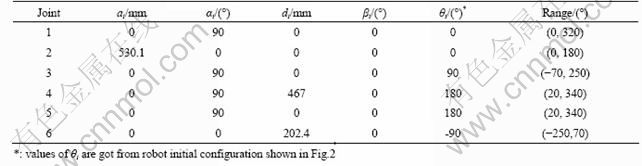
It is well known that the more the measurement poses used to calibration process, the more accurate the pose of end-effector can be achieved. However, the singular value decomposition is a time-consuming work. A large number of measurement poses will bring a large size identification Jacobian matrix which seriously complicates the calculation of SVD. As a result, the optimal problem of pose number comes out. Ordinarily, there are two steps to finish this job. At first, initial n optimal poses should be ascertained. NATEGH and AGHELI [14] selected these poses from the boundary of robot workspace. However, as indicated, for serial robots, the poses located on the boundary are not always optimal to robot calibration. For example, the maximum z value boundary pose is a singular configuration of the six-DOF serial robot introduced in this work. From Fig.3, obviously, this is not an optimal pose for robot calibration. Therefore, at the first step, a modified DETMAX algorithm is used to choose the initial optimal pose set. The (n+1)-th to M-th robot pose is then selected and added to the preliminary n poses by maximizing one kind of observability indices step by step. Usually, M is given a larger value to see a longer change of observability index with respect to robot poses.

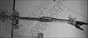
Fig.3 Maximum z value boundary pose of SLIMA

The method utilized above to add poses to the preliminary n poses is called PoseAdded algorithm. It returns a pose which can maximize the observability index of the pose set composed of the original pose set and this added pose. To optimize a pose set, another algorithm called PoseRemoved is also needed. It also returns a pose which can maximize the observability index of the pose set without this pose. Conventions used in both algorithms are defined as follows.

1) Ω is the candidate pose set pool. It includes a number of N poses.

2) n donates the initial pose set number.

3) M_O is the optimal number of measurement poses.

4)  indicates a pose set including n poses which should be modified by the PoseAdded method.

5) P_a is a robot configuration chosen by the PoseAdded algorithm.

6) S_U includes U poses which are randomly selected from Ω. It is used in the PoseAdded method as a candidate pose set. The method will then select an optimal pose from this pose set.

7)  indicates a pose set of n+1 poses which consists of  and P_a.

8) P_r represents a pose that should be removed from  by the PoseRemoved algorithm.

9)  donates the pose set remained after removing P_r from .

The PoseAdded algorithm picks up one pose from S_U each time to add with the pose set  and calculates one kind of observability index of identification Jacobian of the new pose set. Finally, an optimal robot pose P_a that can maximize the index value of the new pose set is selected.

On the contrary, the PoseRemoved algorithm calculates the observability indices each time when a pose belonging to  is removed. At last, a pose P_r corresponding to the maximum index value of a new  is removed from .

Using the combination of the exchange-add- exchange pose selection method and the optimal number obtained above, an optimal set of robot measurement configuration can be acquired. Specifically, the procedure can be shown as follows.

Step 1 (Optimize pose number): As indicated previously, the optimal number of measurement configurations can be confirmed as the foundation of the following steps at first.

Step 2 (Initialize): A number of N measurement configurations are chosen as candidate configurations, and the set of them is named the candidate configuration pool Ω. An initial n robot poses are selected randomly from Ω.

Step 3 (Exchange): The PoseAdded and PoseRemoved method are included in each exchange step. At first, a pose selected from the pose set S_U is obtained by the PoseAdded algorithm to combine with  and create a new set . The PoseRemoved method is then used on the pose set  to exclude one pose from it which affects the index value of  minimally. This step stops when the added pose P_a is consequently removed.

Step 4 (Add): The PoseAdded method is used to add one optimal pose to the pose set obtained in the last exchange step every time until the pose set number exceeds a predefined maximum number M.

Step 5 (Exchange): It is the same as Step 3. It also stops when the added pose P_a is consequently removed.

5 Simulation

It is noteworthy that the kinematic parameter errors made by the errors in manufacturing or assembly are invariable after a robot has been assembled. The geometric calibration is just a process to find them out by using the redundant measurements of robot poses. In reality, the real robot pose under the error parameters can be obtained by the outside measurement sensors like camera or laser interferometer. The geometric errors can then be identified by the method proposed. However, the measurement of the information of robot end-effector poses is impossible during the simulation. Since the error geometric parameters are not known before the calibration, researchers usually choose independent normal distribution random variables as the kinematic parameter errors. In this simulation, the real parameter errors are generated based on the manufacturing and the assembly errors. Specifically, the angle errors are set as 0.014 rad. Length errors are set as 0.8 mm and 2.5 mm. Here, the 2.5 mm-long errors are ?a₂, ?d₄ and ?d₆ just because the values of a₂, d₄ and d₆ are a little large (see Table 1). Adding these errors to the nominal parameters listed in Table 1, the real parameters used in simulation can be acquired. Measurement noises are defined as normal distribution random variables with a mean of 0, a standard deviation of 0.06 for orientation measurement and 0.08 for position. The real and nominal end-effector poses can then be calculated by these real parameters, nominal or design parameters and forward kinematics. Using the identification algorithm proposed, the identified kinematic parameter errors are obtained.

Before applying the optimal algorithm to select the measurement poses, the candidate pose set pool should be settled down firstly. As a result, the pose space is latticed with six grids on each joint angle to generate  46 656 poses for the candidate pool Ω. Here, the candidate pose set S_U for the PoseAdded algorithm equals Ω to completely search the optimal poses.

The optimal number of measurement pose searching method proposed is applied with respect to three different observability indices. The results are shown in Figs.4-6. In Fig.4, the poses are selected based on the increase of O_BM. This is to say, at each time, the pose according to the maximum value of O_BM of the new pose set is chosen. Figure 4 shows the value change of the four observability indices with respect to different pose sets. Like Fig.4, Figs.5 and 6 can also be obtained. The only dissimilarity is the criterion of pose selection. Figure 5 is based on the O_DP, and Fig.6 is based on the O_NH2. It is obvious from all these three figures that the condition number O_DP does not increase very much after about 25 poses. This means that the calibration result would not be improved distinctly when the number of the measurement configurations exceeds 25.

As we know, the goal of the robot calibration is to improve the accuracy of the robot end-effector. Thus, 8-50 robot measurement configurations are used to calibrate the robot. The root mean square (RMS) of three direction position errors with respect to the three axes of the base coordinate frame is indicated in Fig.7. The RMS of the length of the end-effector position error vectors is shown in Fig.8. These two figures show again that the accuracy of the end-effector does not change a lot when the number of the measurement configurations used in calibration exceeds 20. When the number equals 25, the best precision can be obtained.

Fig.4 Observability indices based on criterion O_BM

Fig.5 Observability indices based on inverse of O_DP

Fig.6 Observability indices of robot poses based on O_NH2

Fig.7 RMS of position error after calibration based on measurement of 8-50 configurations

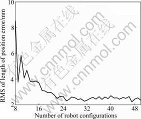
Fig.8 RMS of length of position error vector after calibration by 8-50 configurations

Under the optimal number of end-effector poses, the exchange-add-exchange method is used to get the optimal measurement pose set. The noise amplification index O_NH2 is chosen as the optimal criterion. At first, a pose set including seven poses is randomly selected from the candidate pose pool Ω. Exchange method is used to optimize these seven poses. Keeping implementing the  steps, an optimal pose set can be obtained. This optimal pose set which includes 25 robot poses will then be used in the identification of kinematic parameters. In this work, the least square method is employed to solve the error kinematic model Eq.(11) and retrieve the identified parameters. The geometric parameter errors obtained by the optimal and random pose selection methods and the original parameter error are shown in Fig.9.

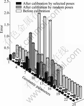
Fig.9 Errors of geometric parameters

Finally, the end-effector pose error after the calibration can be calculated by the identified parameters and forward kinematics. The position and orientation errors yielded by the optimal pose selection method and the random pose selection method are listed in Table 2. ?θ, ?φ and ?ψ are the Euler angle errors of the end-effector with respect to the base coordination frame.

Table 2 Position and orientation errors before and after calibration

As shown in Table 2, the accuracy of end-effector pose after the calibration with the optimal pose selection method proposed in this work is much better than the original one before the calibration. Indeed, the result is better than the calibration with the traditional random pose selection method.

6 Conclusions

1) The optimal number of a pose set for robot calibration is obtained when the value of the observability index, O_DP, does not change distinctly.

2) The exchange-add-exchange pose selection method is implemented evolving the optimal pose number. The calibration based on the optimal pose set obtained by this method can obtain higher end-effector pose accuracy and save time.

3) The simulation on a serial light-weight manipulator with 24 unknown kinematic parameters shows that the end-effector pose accuracy calibrated by using the optimal pose set is much better than the result before the calibration, and is better than that using a random pose set.

References

[1] ROTH Z S, MOORING B W, RAVANI B. An overview of robot calibration [J]. IEEE Journal of Robotics and Automation, 1987, 3(5): 377-385.

[2] BORM J H, MENQ C H. Determination of optimal measurement configurations for robot calibration based on observability measure [J]. International Journal of Robotics Research, 1991, 10(1): 51-63.

[3] DRIELS M R, PATHRE U S. Significance of observation strategy on the design of robot calibration experiments [J]. Journal of Robotic Systems, 1990, 7(2): 197-223.

[4] MENQ C H, BORM H J, LAI J Z. Identification and observability measure of a basis set of error parameters in robot calibration [J]. Journal of Mechanisms, Transmissions, and Automation in Design, 1989, 111(4): 513-518.

[5] NAHVI A, HOLLBERBACH J M, HAYWARD V. Calibration of a parallel robot using multiple kinematic closed loops [C]// Proceedings of the 1994 IEEE International Conference on Robotics & Automation. San Diego, 1994: 407-412.

[6] NAHVI A, HOLLERBACH J M. The noise amplification index for optimal pose selection in robot calibration [C]// Proceedings of the 1996 IEEE International Conference on Robotics & Automation. Minneapolis, 1996: 647-654.

[7] ZHUANG Han-qi, WANG K, ROTH Z S. Optimal selection of measurement configurations for robot calibration using simulated annealing [C]// Proceedings of the 1994 IEEE International Conference on Robotics & Automation. San Diego, 1994: 393-398.

[8] ZHUANG Han-qi, WU Jie, HUANG Wei-zhen. Optimal planning of robot calibration experiments by genetic algorithms [C]// Proceedings of the 1996 IEEE International Conference on Robotics & Automation. San Diego, 1996: 981-986.

[9] DANEY D, PAPEGAY Y, MADELINE B. Choosing measurement poses for robot calibration with the local convergence method and Tabu search [J]. Internal Journal of Robotics Research, 2005, 24(6): 501-518.

[10] WATANABE A, SAKAKIBARA S, BAN K, SHEN G. A kinematic calibration method for industrial robots using autonomous visual measurement [J]. Annals of the CIRP, 2006, 55(1): 1-6.

[11] LIU Qi, WANG Dong-shu. Optimal measurement configurations for robot calibration based on modified simulated annealing algorithm [C]// Proceedings of the 2008 World Congress on Intelligent Control and Automation. Chongqing, 2008: 2300-2305.

[12] SUN Yu, HOLLERBACH J M. Active robot calibration algorithm [C]// Proceedings of the 2008 IEEE International Conference on Robotics & Automation. Minneapolis, 2008: 1276-1281.

[13] SUN Yu, HOLLERBACH J M. Observability index selection for robot calibration [C]// Proceedings of the 2008 IEEE International Conference on Robotics & Automation. Minneapolis, 2008: 831-836.

[14] REN Xiao-dong, FENG Zu-ren, SU Cheng-ping. A new calibration method for parallel kinematics machine tools using orientation constraint [J]. International Journal of Machine Tools & Manufacture, 2009, 49(9): 708-721.

[15] HUANG Chen-hua, XIE Cun-xi, ZHANG Tie. Determination of optimal measurement configurations for robot calibration based on a hybrid optimal method [C]// Proceedings of the 2008 IEEE International Conference on Information and Automation. Zhangjiajie, 2008: 789-793.

[16] ZHAO Hai-xia, WANG Shou-cheng. Optimal selection of measurement configurations for robot calibration with solis&wets algorithm [C]// Proceedings of the 2007 IEEE International Conference on Control and Automation. Guangzhou, 2007: 2429-2432.

[17] DOLINSKY J U, JENKINSON I D, COLQUHOUN G J. Application of genetic programming to the calibration of industrial robots [J]. Computers in Industry, 2007, 58(3): 255-264.

[18] YU Da-yong, SUN Xi-wei, WANG Yu. Kinematic calibration of parallel robots based on total least squares algorithm [C]// Proceedings of the 2007 IEEE International Conference on Mechatronics and Automation. Harbin, 2007: 789-794.

[19] ZHU Yan-he, YAN Ji-hong, ZHAO Jie, CAI He-gao. Autonomous kinematic self-calibration of a novel haptic device [C]// Proceedings of the 2006 IEEE International Conference on Intelligent Robots and Systems. Beijing, 2006: 4654-4659.

[20] VERL A, BOYE T, POTT A. Measurement pose selection and calibration forecast for manipulators with complex kinematic structures [J]. CIRP Annals-Manufacturing Technology, 2008(1), 57: 425-428.

[21] NATEGH M J, AGHELI M M. A total solution to kinematic calibration of hexapod machine tools with a minimum number of measurement configurations and superior accuracies [J]. International Journal of Machine Tools & Manufacture, 2009, 49(15): 1155-1164.

[22] PENROSE R. A generalized inverse for matrices [J]. Proceedings of the Cambridge Philosophical Society, 1955, 51(3): 406-413.

(Edited by YANG Bing)

Foundation item: Project(2008AA04Z203) supported by the National High Technology Research and Development Program of China

Received date: 2010-05-11; Accepted date: 2010-10-14

Corresponding author: LI Tian, PhD; Tel: +86-451-86402330-825; E-mail: litian1@ovi.com