J. Cent. South Univ. (2016) 23: 1937-1943

DOI: 10.1007/s11771-016-3250-6

Application of camera calibrating model to space manipulator with multi-objective genetic algorithm

WANG Zhong-yu(王中宇)¹, JIANG Wen-song(江文松)¹, WANG Yan-qing(王岩庆)²

1. Key Laboratory of Precision Opto-Mechatronics Technology of Ministry of Education

(Beihang University), Beijing 100191, China;

2. Academy of Opto-Electronics, Chinese Academy of Sciences, Beijing 100094, China

Central South University Press and Springer-Verlag Berlin Heidelberg 2016

Abstract: The multi-objective genetic algorithm (MOGA) is proposed to calibrate the non-linear camera model of a space manipulator to improve its locational accuracy. This algorithm can optimize the camera model by dynamic balancing its model weight and multi-parametric distributions to the required accuracy. A novel measuring instrument of space manipulator is designed to orbital simulative motion and locational accuracy test. The camera system of space manipulator, calibrated by MOGA algorithm, is used to locational accuracy test in this measuring instrument. The experimental result shows that the absolute errors are [0.07,1.75] mm for MOGA calibrating model, [2.88, 5.95] mm for MN method, and [1.19, 4.83] mm for LM method. Besides, the composite errors both of LM method and MN method are approximately seven times higher that of MOGA calibrating model. It is suggested that the MOGA calibrating model is superior both to LM method and MN method.

Key words: space manipulator; camera calibration; multi-objective genetic algorithm; orbital simulation and measurement

1 Introduction

The space manipulator is a most important component of a space station. It ensures the orbital space station working security and stability [1]. As the monitor of a space manipulator, the visual system can guide the space manipulator working and moving as required. Therefore, the higher accuracy the visual system has, the higher precision and easier execution for a space manipulator to locate a target.

The locational accuracy of a visual system is closely associated with the optimized characteristic of its camera calibrating model. For a visual system, its camera model calibration is the 3D metric information extraction of an object in world coordinate system (WCS) from its 2D images in image coordinate system (ICS) based on a mathematical model. Such mathematical model is defined as camera model [2].

The better algorithm we choose, the better the camera model has. Since the camera model of a space manipulator is a non-linear system in most cases, a certain new algorithm should be applied to calibrate its camera model to obtain a high measurement accuracy [3]. Therefore, to ensure that the visual system of a space manipulator has a higher accuracy at the most extent, a better method should be chosen to optimize the parameters of the camera model.

Nowadays, the traditional optimization algorithms applied to visual system are least squares (LS) method, Levenberg-Marqurdt (LM) method, and modified Newton (MN) method. The LS method [4-5] is a simple and common used non-linear optimization algorithm. Unfortunately, its operational precision is inversely proportional to the dimensional number of an equation set. Therefore, it is not a good method to solve an equation set with high dimensions [6]. In addition, LM method [7-8] can optimize a non-linear equation set with few parameters easily and quickly. However, it is hard to solve a non-linear equation set with up to ten parameters. What’s more, MN method [9-10] is a wide range convergence Newton method with less dependence on initial values, which has a good astringency. Nevertheless, it has a low iteration precision for non-linear equation set.

The non-linear camera model of space manipulator is built according to the image-forming rule and space geometry transformational principle of its visual system. To improve the imaging precision of such visual system with non-linear and high dimensions characteristics, the MOGA is picked out to calibrate the non-linear camera model. This model is calibrated by optimizing its camera external parameters for its attractive ability of iteration, global optimization, and high-accuracy. This calibrated model can greatly increase the locational accuracy of space manipulator.

2 Working principle of space manipulator and its visual system

The space manipulator is installed on the core module. It mainly consists of certain numbers of joints, arm extensions, and visual system. The joints are the motion actuators to realize force generation, movement transmission, and mechanical connection. They consist of a servo driver, an actuator, a sensor system, a wire harness management device, a data acquisition system, and other relevant devices. In addition, the arm extensions consist of an upper arm and a forearm [11-13]. Besides, the visual system of space manipulator is responsible for target identification and pose detection, which consists of monocular cameras and binocular cameras.

The structure of a space manipulator and the coordinate transformational relationship of its visual system are built, as shown in Fig. 1. The visual system can rapidly detect a target with information of size, shape, distribution and quantity within the field of view. The visual system, installed both on the upper arm and the forearm, can locate a target with the help of elaborate servo-control system [14-15]. In addition, when reaching a target, the visual system can gain its 3D position and attitude from its image coordinate in camera coordinate system (CCS) according to the rotatory matrix R and transfer vector T [16-17].

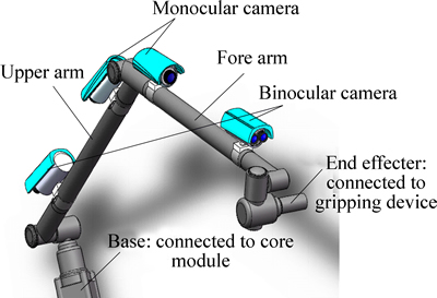
Fig. 1 Physical model of space manipulator

3 Calibration of camera system for a space manipulator

3.1 Non-linear camera model set up

The coordinate transformational model of a visual system between CCS (O_c-X_cY_cZ_c) and ICS (O-uv) based on the mechanical structure of a space manipulator is built, as shown in Fig. 2. The random spatial point P(x_c,y_c, z_c) is imaged by CCD perspective transformation. The mathematical relationship between CCS and ICS is written as follows [18-19],

                              (1)

where f=(a_x, a_y) is the effective focal length of the camera lens. Considering (u₀, v₀) as the center point, the camera model is rewritten as

                              (2)

The mathematical relationship between P(x_w, y_w, z_w) (in WCS) and P(x_c, y_c, z_c) is given by [20]

                          (3)

where is defined as a rotatory matrix, and is defined as a transfer vector. Obviously, the position and attitude of point P projected on CCS is directly determined by the parameters of R and T.

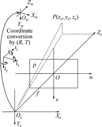
Fig. 2 Transformation from CCS to ICS

By combining Eqs. (2) and (3), we can get

          (4)

where a_x, a_y, u₀ and v₀ are the intrinsic parameters of the camera model, among which a_x and a_y are defined as the effective focal length of axis u and axis v of ICS respectively, (u₀, v₀) is defined as the coordinate of optical center both of ICS and WCS, namely (u₀, v₀) is the center point. From Eq. (4), there are 12 parameters to be solved and those parameters are included in R and T.

3.2 MOGA calibrating model set up

Based on natural selection and evolutionary theory, the MOGA can get the optimal solution of a non-linear objective equation set from its dominant group by artificial evolution, which includes selection, crossover and mutation [21-22]. Generally, the mathematical model of MOGA can be expressed as [23-24]

        (5)

where V-min is stated as the vector minimization; f(x)=[f₁(x), f₂(x), …, f_n(x)]^T is the vector objective function and each sub-function of f(x) is minimized as much as possible.

The six pairs of feature points P_i=(x_wi, y_wi, z_wi) in WCS are picked out to solve Eq. (4), and their corresponding image coordinate is p_i=(u_i, v_i) in ICS. Substitute those six pairs of feature points into Eq. (4), we have

        (6)

where, the external parameters to be solved in Eq. (6) are X=[r₁, r₂, …, r₉, t_x, t_y, t_z], and i=1, 2, …, 6. Furthermore, according to Eq. (6), we have in summary

(7)

Obviously, Eq. (7) is the non-linear camera model to be calibrated, namely, the optimal solution of X can be solved by optimizing Eq. (7). It can be shortened to

Find:           (8)

Min:                  (9)

where Ψ is stated as the solution domain, and X is the optimal solution once F(X)=0.

There are five steps to calibrate the non-linear camera model by MOGA, as shown in Fig. 3.

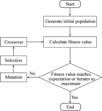
Fig. 3 Flow of MOGA calibration

Step 1) Set the decision variable r₁, r₂, …, r₉, t_x, t_y, t_z, and its constraint condition, namely, (j=1, 2, …, 12). X_j is the initial iterative values and h is the corresponding step size.

Step 2) Set the encoding method of MOGA. The encoding law is the decision variable translation into binary string. The binary string length is determined by the required accuracy of the solution. n is regarded as the decimal places of the solution. m_j for the binary string length can be computed as

              (10)

Step 3) Design the decoding method. The binary string of the decision variable needs to be converted into an effective value, and the conversion formula is given by

  (11)

where decimal(substring_j) is the decimal value of x_j.

Step 4) Build individual evaluate method. The binary string is decoded to effective value before evaluate the fitness of its genome, we can write

, k=1, 2, … (12)

Then, the objective function F(X^(k)) can be evaluated by k times iteration, and its fitness function is

              (13)

Step 5) Set the multiple parameters of the non-linear camera model by genetic operation and iteration. Roulette wheel selection (RWS) method is used for select operation to build a new population by probability. In addition, the crossover operator generates new candidate offspring by recombining the genetic information gained from the selected parent chromosomes. On this occasion, basic bit mutational strategy is chosen as the mutative operation, namely, if the gene is 1, we mutate it to 0; otherwise, set it to 1. Finally, the optimized external parameters X=[r₁, r₂, …, r₉, t_x, t_y, t_z] can be solved by evaluating the fitness curve when iterative process is over.

4 Experimental design and discussion

4.1 Experimental realization

The selected example of a space manipulator, is a model machine for the ground test, illustrates the application advantages of the MOGA calibrating model. The measuring instrument of the space manipulator is a ground experimental system to simulate the orbital measurement, as shown in Fig. 4. The measuring instrument consists of a space manipulator, a guide rail, a simulated core module, and a coordinate measuring machine (CMM and its precision is ±0.002 mm). Our designed space manipulator is fixed on the simulated core module to ensure the test process stability as well as to against vibration. The CMM, is installed on the guide rail, simulates the relative orbital motion between space manipulator and the cooperative target. The cooperative target array is distributed on the destination adapter with several characteristic points. The destination adapter with 6 DOF is installed on the fixed head of CMM. The varied coordinate of a cooperative target can be tested by CMM timely when it drives the destination adapter moving. Meanwhile, this varied coordinate will be also detected by the calibrated camera model of the visual system of space manipulator.

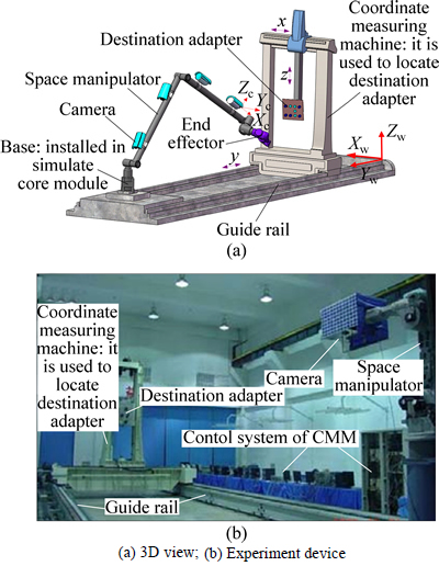
Fig. 4 Measuring instrument of space manipulator:

There are three steps required in this orbital experiment:

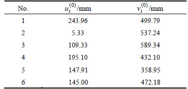
Step 1) Model initialization.are solved by the initial value of X⁽⁰⁾, the six pairs of points P_i, and the camera intrinsic parameters based on Eq.(4) and Table 1, as listed in Table 2.

Table 1 Initial values of non-linear camera model

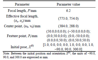
Table 2 Image coordinates calculated by initial values

Step 2) Target detection. The world coordinates of those five feature points on the destination adapter are tested by CMM, i.e. point #a with P_a(x_a, y_a, z_a), point #b with P_b(x_b, y_b, z_b), point #c with P_c(x_c, y_c, z_c), point #d with P_d(x_d, y_d, z_d), and point #e with P_e(x_e, y_e, z_e). The points #a, #b, #c, #d and #e are also tested by the calibrated visual system of space manipulator. Their image coordinates are P_a(u_a, v_a), P_b(u_b, v_b), P_c(u_c, v_c), P_d(u_d, v_d) and P_e(u_e, v_e), respectively. The corresponding world coordinates are …,

Step 3) Result comparison. The world coordinates of those five feature points solved both by CMM and the calibrated visual system are compared respectively to verify the accuracy of different calibrating model.

4.2 Result and discussion

Figure 5 shows the fitness function curve of the MOGA calibrating model after 200 times iteration. It can be seen that the fitness function becomes gradually stable when iteration continues.

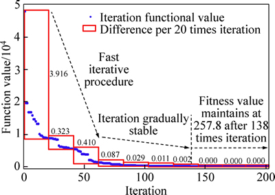
Fig. 5 Fitness curve of MOGA

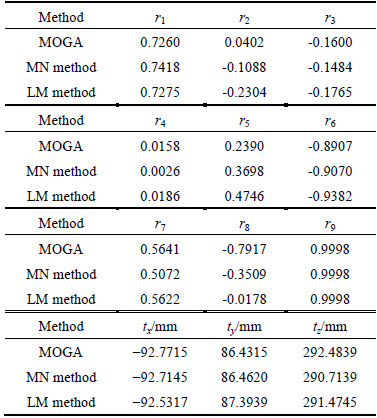
As the best fitness value, X⁽¹³⁸⁾ is the optimal solution of the non-linear camera model because the fitness value maintains at 257.8 after 138 times iteration. The non-linear camera model is also optimized both by MN method and LM method respectively to get the calibrated visual system. All the optimal solutions X^(k) are solved, as listed in Table 3.

Table 3 Comparison of optimal solutions

Substituting the optimal solutions X^(k) into Eq. (4), we can get the optimized image coordinates p_i. The result distribution calibrated by different method is compared in ICS, as shown in Fig. 6. Those points in the same orange circle are the same point calibrated by different methods. It can be seen that those optimal points are quite close partly.

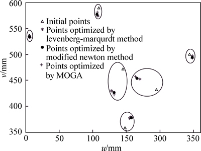
Fig. 6 Distribution of image coordinates

To explain the closeness of those optimal points, the relative error δ_r between each two calibrating methods is defined, which is denoted by [25-26]

                        (14)

where x₁ is the coordinate value of both u_i and v_i calibrated by a method, while x₂ is the coordinate value both of u_i and v_i calibrated by another method.

The relative error δ_r for each two calibrating methods is compared, as shown in Fig. 7. Obviously, it shows that the relative error ranges are only within [-0.1470, 0.038] for u_i, and [-0.011, 0.019] for v_i. It means that every calibrating model can get the real points in the rough scope of true values.

To compare the accuracy of the camera calibrating model optimized by different methods, five feature points on a destination adapter are applied to experiment, as described by step 2, step 3, and step 4 in Section 3.1. The world coordinates are solved, as Table 4 shows.

Since the accuracy of CMM is higher than that of the visual system of space manipulator, P(x, y, z) is stated as the true value. P′(x′, y′, z′), solved by different calibrating model, is stated as the experimental result. The absolute error δ between experimental result and true value can be written as

                  (15)

Figure 8 shows the 3D absolute error of those calibrating models. The absolute error ranges are [2.88, 5.95] mm for MN method, [1.19, 4.83] mm for LM model, and [0.07, 1.76] mm for MOGA calibrating model. It indicates that the MOGA calibrating model has a higher accuracy than other two models.

Fig. 7 Relative error comparison of different calibrating method: _i

Table 4 Comparison between experimental results and true values of feature points

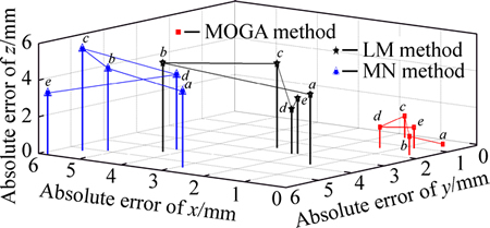
Fig. 8 Absolute errors of calibrated models

The composite errors of those methods are evaluated by root mean square error (RMSE), which works by measuring the total deviation between the experimental value and the true value. Hence, the composite error can be denoted by

 (16)

where δ_x, δ_y and δ_z are the absolute errors of world coordinate components, x, y and z axis; r_(x,y), r_(x,z), and r_(y,z) are the correlative coefficient between each two world coordinate components. The traditional method of mathematical statistics can evaluate the correlation coefficient based on the array of true values.

(x_i, y_i, z_i) is assumed as the experimental result of a certain dot. The correlative coefficient r_(x,y) between x axis and y axis can be defined as follows [27-28]:

              (17)

where n is the test number; i=1, 2, …, n. Similarly, r_(x,z) and r_(y,z) can also be solved by Eq. (17). r_(x,y)=0.25, r_(x,z)=0.05 and r_(y,z)=0.64 are solved respectively.

The composite errors of those calibrating methods are solved by Eq. (16), as shown in Fig. 9. It can be seen that the composite errors are only [0.87, 2.89] mm for MOGA calibrating model. However, the composite errors are [9.04, 11.97] mm for MN method, and [5.75, 9.95] mm for LM method. It indicates that the composite errors both of LM method and MN method are approximately seven times that of MOGA calibrating model.

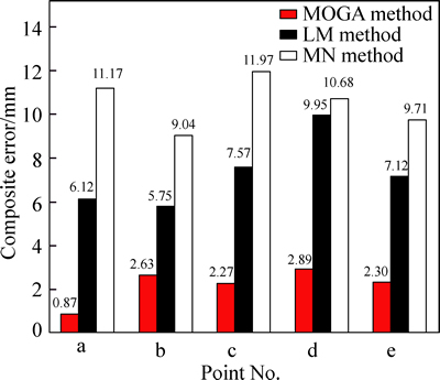
Fig. 9 Composite errors of calibrated models

5 Conclusions

1) For optimal points in ICS, the relative error ranges are [-0.147, 0.038] for u_i, and [-0.011, 0.019] for v_i. It means that the MOGA calibrating model, MN method, and LM method are able to get the real point in the rough scope of true value.

2) When locating the feature points, the absolute error ranges are [0.07, 1.75] mm located by MOGA calibrating model, [2.88, 5.95] mm located by MN method, and [1.19, 4.83] mm located by LM method. It implies that the absolute error range of MOGA calibrating model is much smaller than that both of MN method and LM method.

3) The composite errors are [0.87, 2.89] mm for MOGA calibrating model, [5.75, 9.95] mm for LM method, and [9.04, 11.97] mm for MN method. It indicates that the composite errors both of LM method and MN method are approximately seven times that of MOGA calibrating model. In all, the MOGA calibrating model has a higher accuracy than other two methods when it comes to feature point’s location. The MOGA is superior both to MN method and LM method for the non-linear camera model calibration of space manipulator.

References

[1] BOWSKA E, PIETRAK K. Constrained mechanical systems modeling and control: A free-floating space manipulator case as a multi-constrained system [J]. Robotics and Autonomous Systems, 2014, 62: 1353-1360.

[2] MARCO S, RICCARDO M, PAOLO G. Deployable space manipulator commanded by means of visual-based guidance and navigation [J]. Acta Astronautica, 2013, 83: 27-43.

[3] CHIARA T, MARCO S, PAOLO G. Optimal target grasping of a flexible space manipulator for a class of objectives [J]. Acta Astronautica, 2011, 68: 1031-1041.

[4] PEYMAN H. First order system least squares method for the interface problem of the Stokes equations [J]. Computers & Mathematics with Applications, 2014, 68: 309-324.

[5] ARGYROS I, A. Local convergence analysis of proximal Gauss–Newton method for penalized non-linear least squares problems [J]. Applied Mathematics and Computation, 2014, 241: 401-408.

[6] CARLOS R, ANTONIO J. Robust metric calibration of non-linear camera lens distortion [J]. Pattern Recognition, 2010, 43: 1688-1699.

[7] PAULA M, JUNG C, SILVEIRA J. Automatic on-the-fly extrinsic camera calibration of onboard vehicular cameras [J]. Expert Systems with Applications, 2014, 41: 1997-2007.

[8] SHIRKHANI R. Modeling of a solid oxide fuel cell power plant using an ensemble of neural networks based on a combination of the adaptive particle swarm optimization and Levenberge Marquardt algorithms [J]. Journal of Natural Gas Science and Engineering, 2014, 21: 1171-1183.

[9] HUESO J, E, TORREGROSA R. Modified Newton’s method for systems of non-linear equations with singular Jacobian [J]. Journal of Computational and Applied Mathematics, 2009, 224: 77-83.

[10] LIANG Fang. A modified Newton-type method with sixth-order convergence for solving non-linear equations [J]. Procedia Engineering, 2011, 15: 3124-3128.

[11] LUO Zai, JIANG Wen-song, GUO Bin, LU Yi. Analysis of separation test for automatic brake adjuster based on linear radon transformation [J]. Mechanical Systems and Signal Processing, 2015, 50: 526-534.

[12] FERNANDO L, ANTONIO C, HSUT L. Adaptive visual servoing scheme free of image velocity measurement for uncertain robot manipulators [J]. J Automatica, 2013, 49: 1304-1309.

[13] MARCO S, RICCARDO M, PAOLO G. Adaptive and robust algorithms and tests for visual-based navigation of a space robotic manipulator [J]. Acta Astronautica, 2013, 83: 65-84.

[14] Z, MARKO M, MIHAILO L. Neural network reinforcement learning for visual control of robot manipulators [J]. Expert Systems with Applications, 2013, 40: 1721-1736.

[15] MOHAMMAD J, MOHAMED F, MOHAMMAD N. Automatic control for a miniature manipulator based on 3D vision servo of soft objects [J]. Mechatronics, 2012, 22: 468-480.

[16] ZHANG Xiu-ling, ZHAO Liang, ZANG Jia-yin. Visualization of flatness pattern recognition based on T-S cloud inference network [J]. Journal of Central South University, 2015, 22: 560-566.

[17] DARIUSZ R, P. Software application for calibration of stereoscopic camera setups [J]. Metrology and Measurement Systems, 2012, 19: 805-816.

[18] THANH HAI T, FLORENT R, C. Camera model identification based on DCT coefficient statistics [J]. Digital Signal Processing, 2015, 40: 88-100.

[19] SUN Jun-hua, XU Chen, ZHENG Gong. Accurate camera calibration with distortion models using sphere images [J]. Optics & Laser Technology, 2014, 65: 83-87.

[20] TARIK E, ADLANE H, BOUBAKEUR B. Self-calibration of stationary non-rotating zooming cameras [J]. Image and Vision Computing, 2014, 32: 212-226.

[21] SENTHILNATH J, NAVEEN K, BENEDIKTSSON A. Accurate point matching based on multi-objective genetic algorithm for multi-sensor satellite imagery [J]. Applied Mathematics and Computation, 2014, 236: 546-564.

[22] de ARRUDA P, DAVIS C, GONTIJO C. A niching genetic programming-based multi-objective algorithm for hybrid data classification [J]. Neuro-computing, 2014, 133: 342-357.

[23] ZHAO Xin, CHEN Cheng, MA Nin. Alternating direction method of multipliers for non-linear image restoration problems [J]. IEEE Transactions on Image Processing, 2014, 99: 1.

[24] MAHMOODABADI M, TAHERKHORSANDI M, BAGHERI A. Optimal robust sliding mode tracking control of a biped robot based on ingenious multi-objective PSO [J]. Neurocomputing, 2014, 124: 194-209.

[25] ZHANG Xiao-hu, ZHU Zhao-kun, YUAN Yun. A universal and flexible theodolite-camera system for making accurate measurements over large volumes [J]. Optics and Lasers in Engineering, 2012, 50: 1611-1620.

[26] WANG Zhong-yu, LIU Zhi-min, XIA Xin-tao. Measurement error and uncertainty evaluation [M]. Beijing: Science Press, 2008: 62-65. (in Chinese)

[27] CHEN C C, HUI M, BARNHART X. Assessing agreement with intraclass correlation coefficient and concordance correlation coefficient for data with repeated measures [J]. Computational Statistics & Data Analysis, 2013, 60: 132-145.

[28] CHUHO Y, SHIN Y, CHO J. Visual attention and clustering-based automatic selection of landmarks using single camera [J]. Journal of Central South University, 2014, 21: 3525-3533.

(Edited by YANG Hua)

Foundation item: Project(J132012C001) supported by Technological Foundation of China; Project(2011YQ04013606) supported by National Major Scientific Instrument & Equipment Developing Projects, China

Received date: 2015-06-08; Accepted date: 2015-12-10

Corresponding author: WANG Zhong-yu, Professor, PhD; Tel: +86-13691536014; E-mail: mewan@buaa.edu.cn