Wafer bin map inspection based on DenseNet
��Դ�ڿ������ϴ�ѧѧ��(Ӣ�İ�)2021���8��
�������ߣ����˹� ���� ����½ �ּ�
����ҳ�룺2436 - 2450
Key words��wafer defect inspection; convolutional neural network; DenseNet; model uncertainty
Abstract: Wafer bin map (WBM) inspection is a critical approach for evaluating the semiconductor manufacturing process. An excellent inspection algorithm can improve the production efficiency and yield. This paper proposes a WBM defect pattern inspection strategy based on the DenseNet deep learning model, the structure and training loss function are improved according to the characteristics of the WBM. In addition, a constrained mean filtering algorithm is proposed to filter the noise grains. In model prediction, an entropy-based Monte Carlo dropout algorithm is employed to quantify the uncertainty of the model decision. The experimental results show that the recognition ability of the improved DenseNet is better than that of traditional algorithms in terms of typical WBM defect patterns. Analyzing the model uncertainty can not only effectively reduce the miss or false detection rate but also help to identify new patterns.
Cite this article as: YU Nai-gong, XU Qiao, WANG Hong-lu, LIN Jia. Wafer bin map inspection based on DenseNet [J]. Journal of Central South University, 2021, 28(8): 2436-2450. DOI: https://doi.org/10.1007/s11771-021-4778-7.

J. Cent. South Univ. (2021) 28: 2436-2450
DOI: https://doi.org/10.1007/s11771-021-4778-7

YU Nai-gong(���˹�)1, 2, 3, XU Qiao(����)1, 2, 3, WANG Hong-lu(����½)1, 2, 3, LIN Jia(�ּ�)1, 2, 3
1. Faculty of Information Technology, Beijing University of Technology, Beijing 100124, China;
2. Beijing Key Laboratory of Computing Intelligence and Intelligent System, Beijing 100124, China;
3. Engineering Research Center of Digital Community, Ministry of Education, Beijing 100124, China
 Central South University Press and Springer-Verlag GmbH Germany, part of Springer Nature 2021
Abstract: Wafer bin map (WBM) inspection is a critical approach for evaluating the semiconductor manufacturing process. An excellent inspection algorithm can improve the production efficiency and yield. This paper proposes a WBM defect pattern inspection strategy based on the DenseNet deep learning model, the structure and training loss function are improved according to the characteristics of the WBM. In addition, a constrained mean filtering algorithm is proposed to filter the noise grains. In model prediction, an entropy-based Monte Carlo dropout algorithm is employed to quantify the uncertainty of the model decision. The experimental results show that the recognition ability of the improved DenseNet is better than that of traditional algorithms in terms of typical WBM defect patterns. Analyzing the model uncertainty can not only effectively reduce the miss or false detection rate but also help to identify new patterns.
Key words: wafer defect inspection; convolutional neural network; DenseNet; model uncertainty
Cite this article as: YU Nai-gong, XU Qiao, WANG Hong-lu, LIN Jia. Wafer bin map inspection based on DenseNet [J]. Journal of Central South University, 2021, 28(8): 2436-2450. DOI: https://doi.org/10.1007/s11771-021-4778-7.
1 Introduction
The semiconductor manufacturing process is complex, precise and requires multiple processes, such as film deposition, etching, polishing, scribing, and inversion. Any abnormality in the process may cause wafer defects and affect the product yield. In recent years, competition in the chip manufacturing industry has become fierce, reducing costs and improving quality via lean production are crucial factors maintaining the competitiveness of enterprises [1]. Wafer bin map (WBM) inspection is an important way to control the semiconductor yield. When a fault exists in the process, the defective grains tend to aggregate into a certain distribution pattern that can track the detailed fault information. However, limited by the precision and machine learning ability of automatic systems, the inspection operation still relies on manual analysis, with high labor intensity and low efficiency. Therefore, high-precision and intelligent inspection equipment is needed.
Figure 1 shows the typical WBM defect patterns in the WM811K wafer dataset, including Center, Donut, Edge-Loc, Edge-Ring, Loc, Random, Scratch, Near-Full and None patterns. The dataset is derived from the real wafer probe test in the manufacturing process. WBM defect patterns reflect important information about the production process. For instance, the Edge-Ring pattern was caused by temperature control anomalies during annealing, and the Scratch pattern was caused by mechanical polishing or cutting anomalies. According to the causes of defects, the WBM defect patterns can be divided into random defects and system defects [2]:
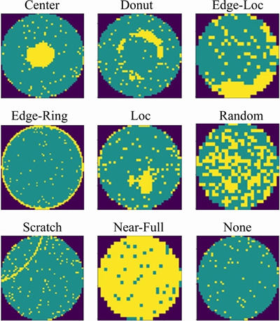
Figure 1 Typical WBM defect patterns in WM811K wafer dataset
Random defects: Defects are caused by random factors in the production environment. Similar to the None pattern in Figure 1, the defective grains do not aggregate into a certain spatial distribution, but a mass of defective grains still exist. Random defects cannot be completely eliminated, however, improving the process may help to reduce the densities of the defective grains.
System defects: These defects are caused by operating errors or abnormal equipment. Defective grains have certain spatial distribution patterns, such as the first 8 defect patterns in Figure 1.
Traditional WBM inspection methods are based on image processing and machine learning. However, these methods require manual selection of features and parameters. With the development of the manufacturing process, new defect patterns have been continuously increasing. Features have high similarity, so traditional visual processing approaches have been unable to satisfy the dynamic and complex production environment. The development of deep learning technology in computer vision tasks promotes the progress of automatic optical inspection, but the structure of neural networks limits the generalization capability to new categories. In addition, decision reliability is crucial for evaluating the performance of fault diagnosis systems. In many cases, we need to know the confidence of prediction to avoid the nondetection and misdetection; however, the traditional methods do not consider it.
This paper introduces a WBM defect pattern inspection strategy and conducts training and testing on the WM811K wafer dataset. First, a constrained mean filtering algorithm is proposed to preprocess the WBM. Second, to solve the problem of unbalanced training samples and indistinguishable features, the structure and loss function of DenseNet are optimized, so that the average recognition accuracy for Center, Donut, Edge-Loc, Edge-Ring, Loc, Random, Scratch, Near-Full and None patterns achieves 91.5%. Last, we integrate the entropy-based Monte Carlo dropout into DenseNet to evaluate the decision reliability, and the classification error rate is further reduced by 2.16%.
The remainder of the paper is organized as follows: Section 2 shows the related work; Section 3 introduces the details of the improved DenseNet model; Section 4 describes the experimental results and Section 5 gives the conclusion.
2 Related work
According to the dependence on training data, WBM inspection can be divided into unsupervised learning and supervised learning, among which deep learning is a trend of research in recent years.
2.1 Unsupervised learning
Due to the difficulty in obtaining and marking defective wafers, unsupervised learning was adopted. CHEN et al [3] employed adaptive resonance theory (ART) to perform cluster analysis of the WBM and judged the pattern by similarity. However, the number of defect patterns recognized by ART is limited. WANG et al [4] proposed a Gaussian expectation maximization algorithm to estimate ellipses and linear defect clusters. HWANG et al [5] improved WANG��s work by a model-based clustering analysis algorithm that modeled ellipsoid and linear defects using binary normal distribution, and described the curve pattern using the main curve. Based on statistical analysis, these methods can estimate basic linear, ellipse, curve and ring defect clusters, but cannot adapt to more complex defect patterns in the current production process. YU et al [6] reduced the dimension of defect cluster features based on manifold learning and constructed a defect library by the Gaussian mixture model. The proposed method could identify unknown defect patterns and obtained an average accuracy of 90.5% with the WM811K dataset. Different from the previously described, JIN et al [7] fully considered defect grains, did not eliminate random defects, and simultaneously extracted defect cluster patterns and detected outliers. They proposed a density-based clustering method that can be applied to the classification of mixed defect patterns. Other unsupervised learning approaches include K-means [8], hierarchical clustering [9], neural network clustering [10], dominant defective patterns finder [11], etc. In addition, semi-supervision [12] and active learning [13] have also been applied. The unsupervised clustering algorithm relies on the distance of the space characteristics and is not suitable for specific pattern classification. With the accumulation of data and labeling, supervised training is not an obstacle and greatly improves the recognition accuracy.
2.2 Supervised learning
Supervised learning mainly relies on training data to adjust the model parameters. PIAO et al [14] applied a decision tree ensemble algorithm to realize WBM failure pattern recognition (DTE-WMFPR) based on the Radon feature, which was able to identify new defect categories. SAQLAIN et al [15] presented an integrated learning scheme with multi-classifiers to learn the geometry, Radom and density features of WBMs. In addition, support vector machine (SVM) [16] and neural network [17] are also common choices for traditional WBM inspection. However, traditional methods combine image processing algorithms with machine learning classifiers. The disadvantages of traditional approaches are that effective features need to be selected manually and more parameters need to be adjusted. Therefore, the classification accuracy is unsatisfactory and the implementation process is complex.
In recent years, deep learning technology has made unprecedented progress in the field of computer vision and also provides a new solution for fault detection system [18]. NAKAZAWA et al [19] proposed applying a 5-layer convolutional neural network (CNN) to classify WBM defect patterns. In literature [20], they further proposed a deep convolutional encoding-decoding architecture to segment defect regions, which laid a foundation for feature learning. DEVIKA et al [21] trained an 8-layer CNN model to identify four types of defect patterns and their combinations. SHEN et al [22] introduced transfer learning and applied the typical DenseNet-169 (T-DenseNet) network, which has been pretrained to detect the WBM. However, due to the excessively deep level of the original network, the identification effect of Center and Random patterns was weak. To avoid interference from the background, WANG et al [23] mapped the WBM into a matrix through polar coordinates and then input it into CNN, achieving 90% accuracy. The imbalance of the dataset directly affects the performance of the model. SAQLAIN et al [24] applied data augmentation using random rotation, horizontal flipping, width shift, height shift, shearing range and channel shifting, while MAKSIM trained a deep convolutional neural network (DCNN) via the synthesized wafer dataset, which was well verified with the real WBM dataset [25]. It is worth noting that the accuracy of the deep learning methods is improved, but the structure of the CNN limits the discovery of new categories during testing. CHEON et al [26] developed a method that combines K nearest neighbor (KNN) with the CNN. The defect feature was extracted by the CNN, and the new defects were identified by the KNN. The method was applied to the scanning electron microscope detection of grains. However, this approach is not end-to-end and increases the model complexity.
CNN is satisfactory at extracting the deep semantic information of images and is an end-to-end classifier. However, the structure of deep neural networks limits the generalization of new categories. The semantic information of the WBM is weak, and the deep network will lead to the loss of shallow layer information. Typical models, such as VGG [27], ResNet [28], and DenseNet [29], are deepening the network. Therefore, how to choose and improve the deep learning model is also an important issue.
2.3 Model uncertainty
As previously mentioned, identifying new defect categories (which never appear in the training set) is difficult with deep learning. The CNN-KNN strategy proposed by CHEON et al [26] undermined the advantages of CNN end-to-end detection. In terms of fault diagnosis systems, an incorrect decision may cause a large economic loss, which can be avoided by uncertainty analysis. Therefore, model uncertainty is introduced in our project, and high decision uncertainty output by the network when meeting new defects. The uncertainty of the deep neural network has always been a problem. Bayesian inference is an effective tool for knowledge inference and uncertainty assessment [30]. As early as 1997, BISHOP [31] explained the application of Bayesian inference in neural networks. The Bayesian neural network considered weight the probability distribution, calculated the posterior distribution according to the input and prior knowledge, and then judged the decision uncertainty based on the prediction variance. However, the calculation of the posterior distribution was awkward. Numerous improved Bayesian neural networks [32-38] have been proposed, among which the effective methods are Markov chain Monte Carlo (MCMC) [32, 33] and variational inference (VI) [35-38]. The MCMC approaches have an immense computational cost. The approximate precision of VI methods was difficult to control and the calculation was large. Although these algorithms had excellent performance in feedforward networks and recurrent neural networks, their application in convolutional neural networks was limited by computation. By theoretical derivation, GAL et al [39] showed that the application of Monte Carlo integration and dropout in neural networks could be applied as a Bayesian approximation of the Gaussian process, which was referred to as the Monte Carlo dropout algorithm. The algorithm solved the problems of large computation and low accuracy, and was well applied in regression [40], classification [41] and reinforcement learning [42]. Our work will also draw on the Monte Carlo dropout algorithm.
3 Methodology
The proposed method can be divided into two stages: offline modeling and online inspection. The overall scheme diagram is shown in Figure 2. The training and testing are based on the WM811K wafer dataset. The input image is preprocessed using a constrained mean filtering algorithm in two stages. In the offline modeling stage, the loss function and structure of DenseNet were optimized and trained on the dataset. In the online inspection phase, the input WBM is predicted by the improved DenseNet, and the decision uncertainty is calculated based on Monte Carlo dropout (MC dropout). If the uncertainty is within an acceptable range, the reliability of the model decision is shown to be strong; otherwise manual analysis is needed.
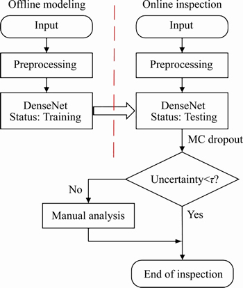
Figure 2 Overall scheme diagram of WBM inspection (Offline modeling stage: optimize and train the DenseNet model. Online inspection stage: recognize the pattern for input WBM and analyze model uncertainty)
3.1 Image preprocessing
The noise of the WBM refers to the random defective grains on it. These grains do not form a certain distribution pattern, which is caused by the production environment and cannot be completely eliminated. For example, the None pattern in Figure 1 shows that a defect cluster does not exist, but there are still random defective grains. Although this kind of noise is allowed in production, it seriously affects the performance of defect pattern recognition.
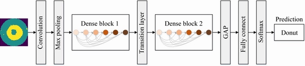
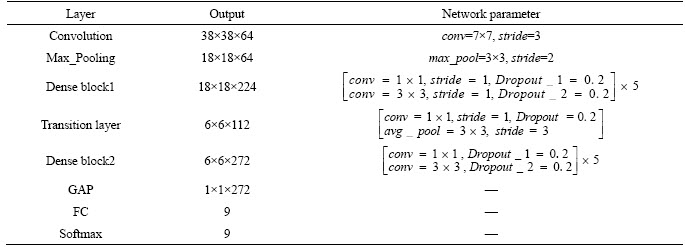
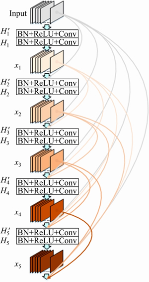
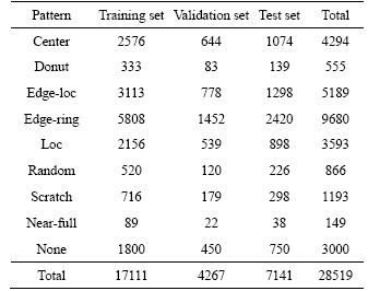
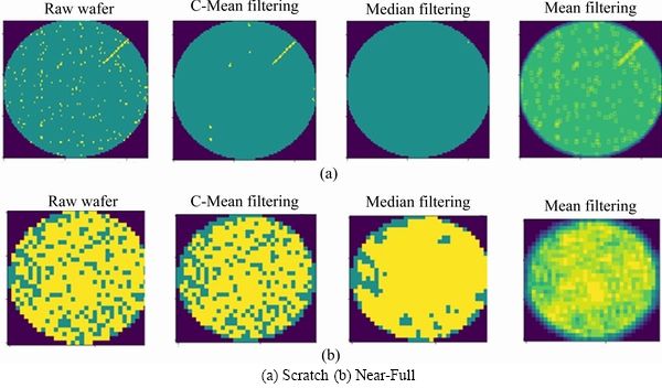
Median filtering [6] is a common method of wafer preprocessing that may cause edge blurring (converting edge grains into the background) or filtering out normal grains (converting normal grains into defects). The purpose of WBM preprocessing is to reduce the influence of random defective grains. Therefore, we propose a constrained mean filtering algorithm, which can only filter defective grains without destroying the edge, effectively protect normal grains and filter random noise. As shown in Figure 3, the WBM has only three meaningful pixel values: background, normal grain and defective grain, Number 0 represents the background, 1 represents the normal grain, and 2 represents the defective grain. We define f(x, y) as the filtering target and define w as the filter window, as shown in the red box in Figure 3. We use w with a size of 3��3 and use k as the number of neighborhood elements. The filtering process is shown in formula (1):
 (1)
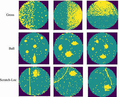
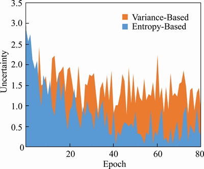
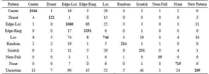
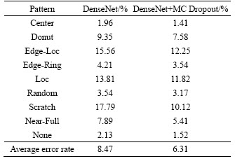
(1)
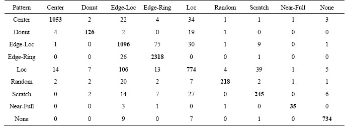
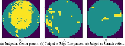
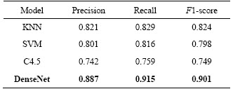
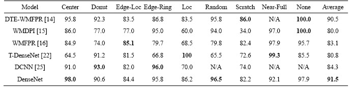
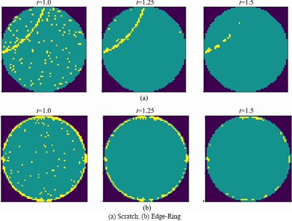
The filter scans matrix elements and leaves the original pixel unchanged when the target element is the background or normal grain. When the target element is a defective grain, the mean g(x, y) of the neighborhood pixels is calculated. To ensure that no extra elements appear in the filtered WBM, the mean results need to be judged again. Define the threshold value t, convert the target element to a normal grain when g(x, y) Figure 3 Wafer data matrix (0 represents background, 1 represents normal grain and 2 represents defective grains) 3.2 DenseNet model With the increasing requirements of computer vision tasks on image semantic features, the convolutional neural network structure is increasingly complex, and the number of parameters is huge. WBM is a simple image, and the shape and location of the defect cluster are important defect patterns. The WBM��s semantic information is weak and texture information is critical. Shallow features are crucial for WBM pattern recognition, and too wide a network or too deep layers will cause the loss of shallow information. Figure 4 Contrast of filtering results with different threshold values t: 3.2.1 DenseNet structure DenseNet [29] is a simple network that focuses on the multiplexing of shallow layers�� features of images. DenseNet references the bypass connection idea of ResNet [28] and combines each feature at the front and back layers into new output instead of superposition. Compared with ResNet, DenseNet has fewer parameters, enhances feature reuse and achieves better performance in the case of low calculation cost. However, the depth of the network is still not suitable for WBM inspection. We pruned the traditional network structure to make the model more concise and efficient. DenseNet is mainly composed of dense blocks, transition layers and fully connected layers. The DenseNet for WBM defect pattern inspection is shown in Figure 5. We adopt two dense blocks, a transition layer, a global average pooling (GAP) layer and a fully connected (FC) layer. The dense connection of the convolution layer is realized in each dense block. The feature map is down-sampled through the transition layer, and the input wafer size is 112��112. Table 1 illustrates the detailed network parameters and outputs. Dense blocks: Two identical dense blocks are employed to learn the defect cluster characteristics of the WBM. Figure 6 shows an internal structure of a dense block that contains five convolutional layers. x represents the feature map and H represents the function composed of the batch normalization (BN), rectified linear units (ReLU), and convolutional layer (Conv). According to formula (2), the input feature maps of layer i are the combined output of previous layers. To ensure the connection of previous feature maps, the outputs of each layer have the same size and there is no pooling layer inside the dense block. In our method, we set the growth rate K=32, which means that convolutional layer outputs 32 feature maps. Since the number of input feature maps increased exponentially after the merge operation, the original DenseNet [29] placed a bottleneck layer in front of each convolutional layer to reduce the network width. We continue this method by adding a 1��1 convolutional layer before convolution operation. The dense blocks ensure the unification size of the feature map, which facilitates the network to realize feature reuse via connection operation, and maintains the network width in an appropriate range through the bottleneck layer. Figure 5 Structure diagram of DenseNet (It composed of dense blocks, convolutional layers, transition layer, global average pooling layer and fully connect layer) Table 1 Detailed decrisption of improved DenseNet Figure 6 Dense Block diagram (output feature map of x1 to x5 is the growth rate K, and K =32. H�� is the bottleneck layer, the 1��1 convolution kernel is adopted; and a 3��3 convolution kernel is applied for function H) Transition layer: It should be noted that only the number of feature maps (network width) is changed in the dense block, and the size of the feature map cannot be changed. Therefore, DenseNet adds a transition layer between the dense blocks to reduce the output size. The transition layer consists of a convolutional layer and an average pooling layer. The convolution layer applies a 1��1 kernel, and the number of output feature maps is half of the input. 3.2.2 Focal loss function As shown in Figure 1, the features of 9 typical WBM defect patterns exhibit different difficulties. For example, patterns such as Donut, Scratch and Edge-Ring have obvious features and are easy to distinguish, while Loc and Center patterns are similar and difficult to distinguish. In addition, the quantity of different categories varies greatly, which causes low efficiency in the training stage. A large number of simple samples will provide too much redundant information to the model. The model should pay more attention to hard samples. LIN et al [43] proposed a dichotomous loss function to solve the unbalanced dataset in the target recognition task, which is a dichotomous loss function. The original expression is as: where y represents the ground truth of the sample and 3.3 Model uncertainty based on MC dropout For WBM inspection, it is inevitable that new defect patterns will appear in the manufacturing process and that undetected or error-detected samples will cause vast economic losses. Since the probability of a new defect is low, we identify it through the uncertainty of the model and address it in the manual analysis. The uncertainty can help people judge the confidence of the model decision which is crucial in fault diagnosis. The traditional neural network is based on maximum likelihood estimation to calculate weight, and the final prediction is estimated by fixed parameters. Therefore, traditional networks often fail to give a reliable confidence and tend to make overconfident wrong decisions. GAL et al [39] showed that the application of the Monte Carlo integration and dropout algorithm in neural networks can be employed as a Bayesian approximation of the Gaussian process, which is named Monte Carlo dropout (MC dropout). Dropout is a random deactivation technique. During iterative training, some of the neurons are randomly closed with a certain probability to improve the generalization ability and reduce overfitting [44]. The MC dropout algorithm turns during training and testing, and the expectation and variance of the T testing results can be taken as the final decision and uncertainty respectively. In terms of time, the execution of T times sampling can be processed in parallel, which is equal to the time of running the model once. For the classification task, the final prediction result is shown in formula (5), and the uncertainty is expressed as formula (6). where x* is the input sample; 4 Experiments and results 4.1 Dataset The proposed model was trained and tested on the WM811K wafer dataset which was collected from the real manufacturing process. There are 811457 samples in the dataset, including 9 WBM defect patterns (Center, Donut, Edge-Loc,Edge-Ring, Loc, Random, Scratch, Near-Full and None), of which only approximately 21% are manually labeled. We randomly divided the labeled samples into a training set, validation set and test set according to the proportion 60%:15%:25%. The detailed division is shown in Table 2. It should be noted that only 3000 None pattern samples were selected for the experiment. Obviously, the dataset is extremely unbalanced, so the Donut, Random, Scratch and Near-Full patterns were extended in the training stage by random rotation and clipping. Table 2 Division of WM811K dataset 4.2 Constrained mean filtering According to the characteristics of the WBM, a constrained mean filtering (C-mean filtering) algorithm was proposed. In this section, we compared the algorithm with the commonly employed median and mean filtering algorithms. The comparison results are shown in Figure 7. A threshold value t of 1.25 was adopted for C-mean filtering, and 3��3 filters were utilized for all the methods. It can be seen that it is easy to destroy the texture feature of the Scratch pattern and lead the partial normal grains to convert into defective grains when using the median filter. The results of the Random pattern after median filtering is similar to those of the Near-Full pattern. The mean filtering yields new pixel values. For the conditions of the same filter size, the C-mean filtering algorithm achieves a better filtering performance. 4.3 Performance of improved DenseNet DenseNet was trained and tested based on the dataset partition in Table 2. A learning rate of 0.001 was adopted, and a total of 80 epochs were iterated. The precision, recall, F1-score, and hybrid matrices were selected to evaluate the model performance. The precision and recall can be expressed by formula (8) and formula (9), respectively. It can be determined that the two evaluation indicators are contradictory, and we need to comprehensively evaluate the performance of the model with the F1-score, as shown in formula (10). Figure 7 Effects of constrained mean filtering (C-mean filtering), median filtering and mean filtering: The influence of �� in the focal loss function was tested and evaluated with the validation set, and an appropriate value was determined using the results in Table 3 where ��=0 represents the traditional cross entropy loss. Obviously, focal loss can make the model pay more attention to feature learning of hard samples and helps to improve the performance of the model. The model recognition ability is best when ��=1. Table 4 shows the classification hybrid matrix for the test set with ��=1. The average accuracy for 9 defect patterns is 91.5%, but the discrimination ability for the Loc pattern is poor. Partial misclassification samples are shown in Figure 8. The main reason for these results is that the feature of the Loc pattern is similar to the Center, Edge-Loc and other patterns, which is difficult to judge even by human observation, which also explains the wrong dataset annotation. Table 3 Influence of �� for model performance on validation set In addition, we compared the model with traditional manual feature extraction methods: KNN, SVM and decision tree. First, we reduced the noise of the WBM based on C-mean filtering. Second, we extracted the texture feature, geometric feature (contour, perimeter, area, and center of defect cluster) and projection feature based on Radom transformation. The KNN algorithm adopted a nearest neighbor coefficient of 1. The linear kernel function was applied in the SVM, and gamma=5. C4.5 was selected for the decision tree algorithm. As seen from the experimental results in Table 5, the recognition rates of the KNN, SVM and C4.5 methods are poor, which shows that the features extracted by the traditional image processing approach are not suitable for describing defect clusters. Compared with traditional feature extraction, DenseNet has a better recognition accuracy for most pattern categories due to CNN��s strong feature extraction and expression ability. The end-to-end approach renders the measurement steps simple. In addition, the end-to-end detection is more concise. Table 4 Classification hybrid matrix for test set Figure 8 Misclassified Loc patterns: Table 5 Performance of KNN, SVM, C4.5 and DenseNet with test set We also perform a comparison with algorithms that have performed well with the WM811K dataset in recent years, including DTE-WMFPR [14], WMDPI [15], WMFPR [16], T-Densenet [22] and the DCNN [25]. To highlight the recognition ability for each defect pattern, we considered the accuracy of each pattern as the evaluation criterion. As shown in Table 6, our improved DenseNet has a better overall recognition rate than the other methods. However, the average accuracy cannot be demonstrated as an acceptable model because each defect is equally important for troubleshooting. The ability of our model to recognize Loc, Scratch,Near-Full and None patterns still lags behind other methods. Next, we further reduced the error rate by analyzing model uncertainty. 4.4 Model uncertainty We introduced an entropy-based MC dropout algorithm to quantify the uncertainty of the DenseNet model. By analyzing the uncertainty, the confidence and reliability of the model decision can be observed and the interpretability can be improved. If the model outputs a high uncertainty, the test sample may be a new defect pattern or misclassified pattern. To evaluate the ability of the model to discover new categories, we introduced three new defect patterns that did not exist in the WM811K dataset, as discussed in literatures [19] and [45]. As shown in Figure 9, the simulation generated patterns are named Gross, Ball and Scratch-Loc, and 100 samples are available for each pattern. During the training stage, the variance-based and entropy-based MC dropout methods were utilized to measure the uncertainty of the validation set. In the experiment, the sampling time T was set to 100, and the running time of the program was equal to the time of sampling once a parallel operation was performed. Dropout at the transition layer was enabled for model testing, and the dropout rate was set to 0.4. Figure 10 illustrates the model uncertainty change during the training stage. The variance-based MC dropout has a slow downward trend and high uncertainty, which may be due to a few extreme values in the prediction. The entropy-based MC dropout performs better than the former and the uncertainty decreases significantly with the optimization of the model. We further analyzed the uncertainty distribution of the validation set, as shown in Figure 11. We drew box diagrams of the wrong prediction and correct prediction samples. The uncertainty distribution of the wrong prediction is wider than that of the correct prediction, and the distribution mean values of the two predictions are approximately 0.577 and 0.508 respectively. In our experiments, 0.577 was selected as the uncertainty threshold �� to recognize new patterns or misclassified samples (uncertainty>��). We evaluated the classification result using the test set by fusing the entropy-based MC dropout method; the classification hybrid matrix is shown in Table 7. For the new defect patterns, the accuracy of the model is 89.67%, the patterns were judged as uncertain samples. For typical defect patterns, there are still 278 samples with high uncertainty, among which 139 are misclassified samples. Table 8 shows the comparison results of the error rates before and after integration of the MC dropout algorithm. By considering the model uncertainty, the error rate of DenseNet is obviously reduced by 2.16%. Table 6 Accuracy comparision of recent classical algorithms on test set (%) Figure 9 Gross, Ball, Scratch-Loc patterns generated by simulation Figure 10 Uncertainty of validation set during training evaluated by variance-based and entropy-based MC dropout algorithms Figure 11 Distribution of uncertainty for correct prediction and wrong prediction 5 Conclusions To solve the problem of the low accuracy and reliability of traditional WBM inspection methods, we propose a strategy based on the improved DenseNet. First, a constrained mean filtering algorithm is presented, which can filter out random noise and retain the critical feature of the WBM. Second, we optimize the DenseNet structure and propose a model that is suitable for WBM defect pattern recognition. Compared with traditional image processing methods, the improved method has a better recognition ability. It should be noted that we focus on the decision uncertainty of the WBM recognition model, which is essential for fault diagnosis systems and has not been considered in previous studies. Calculating the model uncertainty by the integration of the entropy-based MC dropout algorithm in DenseNet can not only identify the new defect pattern but also reduce the classification error rate. Therefore, the decision made by the system is more reliable and confident. Although we have made progress in terms of the recognition accuracy and decision reliability, improvement in our approach is needed. In future research, we will continue to improve the accuracy and focus on the model��s automatic learning ability for few-shot learning of new defect patterns. Contributors YU Nai-gong put forward the conceptualization and core methodology. XU Qiao designed the software and wrote the original draft. WANG Hong-lu conducted the investigation about the related work. LIN Jia was responsible for supervision and provided experimental resources. All authors replied to reviewers�� comments and revised the final version. Conflict of interest YU Nai-gong, XU Qiao, WANG Hong-lu and LIN Jia declare that they have no conflict of interest. Table 7 Hybrid matrix of DenseNet on test set that fuses MC Dropout Table 8 Model error rate comparison before and after MC Dropout algorithm fusion References [1] BERGERET F, LE GALL C. Yield improvement using statistical analysis of process dates [J]. IEEE Transactions on Semiconductor Manufacturing, 2003, 16(3): 535-542. DOI: 10.1109/TSM.2003.815204. [2] HSU S C, CHIEN C F. Hybrid data mining approach for pattern extraction from wafer Bin map to improve yield in semiconductor manufacturing [J]. International Journal of Production Economics, 2007, 107(1): 88-103. DOI: 10.1016/j.ijpe.2006.05.015. [3] CHEN Fei-long, LIU Shu-fan. A neural-network approach to recognize defect spatial pattern in semiconductor fabrication [J]. IEEE Transactions on Semiconductor Manufacturing, 2000, 13(3): 366-373. DOI:10.1109/66.857947. [4] WANG C H, KUO W, BENSMAIL H. Detection and classification of defect patterns on semiconductor wafers [J]. IIE Transactions, 2006, 38(12): 1059-1068. DOI: 10.1080/ 07408170600733236. [5] HWANG J Y, KUO W. Model-based clustering for integrated circuit yield enhancement [J]. European Journal of Operational Research, 2007, 178(1): 143-153. DOI: 10.1016/ j.ejor.2005.11.032. [6] YU Jian-bo, LU Xiao-lei. Wafer map defect detection and recognition using joint local and nonlocal linear discriminant analysis [J]. IEEE Transactions on Semiconductor Manufacturing, 2016, 29(1): 33-43. DOI: 10.1109/TSM.2015. 2497264. [7] JIN Cheng-hao, NA H J, PIAO Ming-hao, POK G, RYU K H. A novel DBSCAN-based defect pattern detection and classification framework for wafer Bin map [J]. IEEE Transactions on Semiconductor Manufacturing, 2019, 32(3): 286-292. DOI: 10.1109/TSM.2019.2916835. [8] CHEN Xiao-yan, ZHAO Chun-dong, CHEN Jian-yong, ZHANG Dong-yang, ZHU Kui-feng, SU Yan-jie. K-means clustering with morphological filtering for silicon wafer grain defect detection [C]// 2020 IEEE 4th Information Technology, Networking, Electronic and Automation Control Conference (ITNEC). Chongqing, China: IEEE, 2020: 1251-1255. DOI: 10.1109/ITNEC48623.2020.9084726. [9] LEE S, KIM D. Distributed-based hierarchical clustering system for large-scale semiconductor wafers [C]//2018 IEEE International Conference on Industrial Engineering and Engineering Management (IEEM). Bangkok, Thailand: IEEE, 2018: 1528-1532. DOI: 10.1109/ IEEM.2018.8607492. [10] CHIEN Chen-fu, HSU S C, CHEN Y J. A system for online detection and classification of wafer Bin map defect patterns for manufacturing intelligence [J]. International Journal of Production Research, 2013, 51(8): 2324-2338. DOI: 10.1080/ 00207543.2012.737943. [11] TAHA K, SALAH K, YOO P D. Clustering the dominant defective patterns in semiconductor wafer maps [J]. IEEE Transactions on Semiconductor Manufacturing, 2018, 31(1): 156-165. DOI: 10.1109/TSM.2017.2768323. [12] KONG Yu-ting, NI Dong. Semi-supervised classification of wafer map based on ladder network [C]// 2018 14th IEEE International Conference on Solid-State and Integrated Circuit Technology (ICSICT). Piscataway, NJ, USA: IEEE, 2018: 1-4. DOI: 10.1109/ICSICT.2018.8564982. [13] SHIM J, KANG S, CHO S. Active learning of convolutional neural network for cost-effective wafer map pattern classification [J]. IEEE Transactions on Semiconductor Manufacturing, 2020, 33(2): 258-266. DOI: 10.1109/TSM. 2020.2974867. [14] PIAO Ming-hao, JIN Cheng-hao, LEE J Y, BYUN J Y. Decision tree ensemble-based wafer map failure pattern recognition based on radon transform-based features [J]. IEEE Transactions on Semiconductor Manufacturing, 2018, 31(2): 250-257. DOI: 10.1109/TSM.2018.2806931. [15] SAQLAIN M, JARGALSAIKHAN B, LEE J Y. A voting ensemble classifier for wafer map defect patterns identification in semiconductor manufacturing [J]. IEEE Transactions on Semiconductor Manufacturing, 2019, 32(2): 171-182. DOI: 10.1109/TSM.2019.2904306. [16] WU Ming-ju, JANG J S R, CHEN J L. Wafer map failure pattern recognition and similarity ranking for large-scale data sets [J]. IEEE Transactions on Semiconductor Manufacturing, 2015, 28(1): 1-12. DOI: 10.1109/TSM.2014.2364237. [17] ADLY F, YOO P D, MUHAIDAT S, AL-HAMMADI Y, LEE U, ISMAIL M. Randomized general regression network for identification of defect patterns in semiconductor wafer maps [J]. IEEE Transactions on Semiconductor Manufacturing, 2015, 28(2): 145-152. DOI: 10.1109/TSM.2015.2405252. [18] LI Zhong-mei, GUI Wei-hua, ZHU Jian-yong. Fault detection in flotation processes based on deep learning and support vector machine [J]. Journal of Central South University, 2019, 26(9): 2504-2515. DOI: 10.1007/s11771-019-4190-8. [19] NAKAZAWA T, KULKARNI D V. Wafer map defect pattern classification and image retrieval using convolutional neural network [J]. IEEE Transactions on Semiconductor Manufacturing, 2018, 31(2): 309-314. DOI: 10.1109/TSM. 2018.2795466. [20] NAKAZAWA T, KULKARNI D V. Anomaly detection and segmentation for wafer defect patterns using deep convolutional encoder�Cdecoder neural network architectures in semiconductor manufacturing [J]. IEEE Transactions on Semiconductor Manufacturing, 2019, 32(2): 250-256. DOI: 10.1109/TSM.2019.2897690. [21] DEVIKA B, GEORGE N. Convolutional neural network for semiconductor wafer defect detection [C]//2019 10th International Conference on Computing, Communication and Networking Technologies (ICCCNT). Kanpur, India: IEEE, 2019: 1-6. DOI: 10.1109/ICCCNT45670. 2019.8944584. [22] SHEN Zong-li, YU Jian-bo. Wafer map defect recognition based on deep transfer learning [C]//2019 IEEE International Conference on Industrial Engineering and Engineering Management (IEEM). Macao, China: IEEE, 2019: 1568-1572. DOI: 10.1109/IEEM44572.2019. 8978568. [23] WANG Rui, CHEN Nan. Defect pattern recognition on wafers using convolutional neural networks [J]. Quality and Reliability Engineering International, 2020, 36(4): 1245-1257. DOI: 10.1002/qre.2627. [24] SAQLAIN M, ABBAS Q, LEE J Y. A deep convolutional neural network for wafer defect identification on an imbalanced dataset in semiconductor manufacturing processes [J]. IEEE Transactions on Semiconductor Manufacturing, 2020, 33(3): 436-444. DOI: 10.1109/TSM. 2020.2994357. [25] MAKSIM K, KIRILL B, EDUARD Z, NIKITA G, ALEKSANDR B, ARINA L, VLADISLAV S, DANIIL M, NIKOLAY K. Classification of wafer maps defect based on deep learning methods with small amount of data [C]// 2019 International Conference on Engineering and Telecommunication (EnT). Dolgoprudny: Russia. IEEE, 2019: 1-5. DOI: 10.1109/EnT47717.2019.9030550. [26] CHEON S, LEE H, KIM C O, LEE S H. Convolutional neural network for wafer surface defect classification and the detection of unknown defect class [J]. IEEE Transactions on Semiconductor Manufacturing, 2019, 32(2): 163-170. DOI: 10.1109/TSM.2019.2902657. [27] SIMONYAN K, ZISSERMAN A. Very deep convolutional networks for large-scale image recognition [C]// 3rd International Conference on Learning Representations. San Diego, CA, United States, 2014. https://arxiv.org/abs/1409. 1556. [28] HE Kai-ming, ZHANG Xiang-yu, REN Shao-qing, SUN Jian. Deep residual learning for image recognition [C]// 2016 IEEE Conference on Computer Vision and Pattern Recognition (CVPR). Las Vegas, NV, USA: IEEE, 2016: 770-778. DOI: 10.1109/CVPR.2016.90. [29] HUANG Gao, LIU Zhuang, VAN DER MAATEN L, WEINBERGER K Q. Densely connected convolutional networks [C]// 2017 IEEE Conference on Computer Vision and Pattern Recognition (CVPR). Honolulu, HI, USA: IEEE, 2017: 2261-2269. DOI: 10.1109/CVPR.2017. 243. [30] MAHMOOD A, TANG Xiao-wei, QIU Jiang-nan, GU Wen-jing, FEEZAN A. A hybrid approach for evaluating CPT-based seismic soil liquefaction potential using Bayesian belief networks [J]. Journal of Central South University, 2020, 27(2): 500-516. DOI: 10.1007/s11771-020-4312-3. [31] BISHOP C M. Bayesian neural networks [J]. Journal of the Brazilian Computer Society, 1997, 4(1). DOI: 10.1590/s0104-65001997000200006. [32] MACKAY D J C. A practical Bayesian framework for backpropagation networks [J]. Neural Computation, 1992, 4(3): 448-472. DOI: 10.1162/neco.1992.4.3.448. [33] BHAT P C, PROSPER H B. Bayesian neural networks [C]// Statistical Problems in Particle Physics, Astrophysics and Cosmology. Oxford, UK: Imperial College Press, 2006: DOI: 10.1142/9781860948985_0032. [34] HERNANDEZ-LOBATO J M, ADAMS R P. Probabilistic backpropagation for scalable learning of Bayesian neural networks [EB/OL] 2015: arXiv: 1502.05336.http//arxiv.org/ abs/1502.05336. [35] SHRIDHAR K, LAUMANN F, MAURIN A L, OLSEN M, LIWICKI M. Bayesian convolutional neural networks with variational inference [EB/OL]. 2018: arXiv: 1806.05978. https://arxiv.org/abs/1806.05978. [36] BLUNDELL C, CORNEBISE J, KAVUKCUOGLU K, WIERSTRA D. Weight uncertainty in neural networks [C]// 32nd International Conference on Machine Learning. Lile, France. 2015. https://arxiv.org/abs/1505.05424. [37] GAL Y, GHAHRAMANI Z. Bayesian convolutional neural networks with bernoulli approximate variational inference [EB/OL]. 2015: arxiv:1506.02158. http://arxiv.org/abs/1506. 02158. [38] ALEX G. Practical variational inference for neural networks [C]// Proceedings of the 25th International Conference on Neural Information Processing Systems. Granada, Spain, 2011. DOI: 10.5555/2986459.2986721. [39] GAL Y, GHAHRAMANI Z. Dropout as a Bayesian approximation: Representing model uncertainty in deep learning [EB/OL]. 2015; arxiv: 1506.02142v4. http://arxiv. org/abs/1506.02142v4. [40] MIOK K. Estimation of prediction intervals in neural network-based regression models [C]//2018 20th International Symposium on Symbolic and Numeric Algorithms for Scientific Computing (SYNASC). Timisoara, Romania: IEEE, 2018: 463-468. DOI: 10.1109/ SYNASC.2018.00078. [41] GHOSHAL B, TUCKER A, SANGHERA B, WONG W L. Estimating uncertainty in deep learning for reporting confidence to clinicians when segmenting nuclei image data [C]// 2019 IEEE 32nd International Symposium on Computer-Based Medical Systems (CBMS). June 5-7, 2019, Cordoba, Spain. IEEE, 2019: 318-324. DOI: 10.1109/CBMS. 2019.00072. [42] LUTJENS B, EVERETT M, HOW J P. Safe reinforcement learning with model uncertainty estimates [C]// 2019 International Conference on Robotics and Automation (ICRA). May 20-24, 2019, Montreal, QC, Canada. IEEE, 2019: 8662-8668. DOI: 10.1109/ICRA.2019.8793611. [43] LIN T Y, GOYAL P, GIRSHICK R, HE K M, DOLLAR P. Focal loss for dense object detection [J]. IEEE Transactions on Pattern Analysis and Machine Intelligence, 2020, 42(2): 318-327. DOI: 10.1109/TPAMI.2018.2858826. [44] SRIVASTAVA N, HINTON G, KRIZHEVSKY A, SUTSKEVER I, SALAKHUTDINOV R. Dropout: A simple way to prevent neural networks from overfitting [J]. Journal of Machine Learning Research, 2014, 15(56): 1929-1958. https://jmlr.org/ papers/v15/srivastava14a.html. [45] LIU Feng. Wafer defects issue study in lithography [D]. Tianjin: Tianjin University, 2012. http://d.wanfangdata.com. cn/thesis/D287523. (in Chinese) (Edited by HE Yun-bin) ���ĵ��� �����ܼ���������ľ�Բͼ��� ժҪ����Բͼ(WBM)����������뵼���������յĹؼ��ֶΣ���Ч�ļ�ⷽ���ܹ���������Ч�����Ʒ���ʡ����������һ�ֻ����ܼ���������ľ�Բͼȱ��ģʽ��ⷽ���������ݾ�Բͼ�ص��ģ�ͽṹ����ʧ���������˸Ľ������⣬�����һ������ֵ�˲��㷨�˳�������������ģ��Ԥ��ʱ�����û����ص����ؿ���Dropout�㷨������ģ�;��ߵIJ�ȷ���ԡ�ʵ�������������ڵ��͵ľ�Բȱ��ģʽ���Ľ�ģ�͵�ʶ���������ڴ�ͳ�㷨��ͨ������ģ�Ͳ�ȷ���ԣ�����������Ч�ؽ���©���ʺ�����ʣ��������ڷ�����ģʽ�� �ؼ��ʣ���Բȱ�ݼ�⣻���������磻�ܼ��������磻ģ�Ͳ�ȷ���� Foundation item: Project(Z135060009002) supported by the Ministry of Industry and Information Technology of China; Project(KZ202010005004) supported by Beijing Municipal Commission of Education and Beijing Municipal Natural Science Foundation of China Received date: 2020-06-10; Accepted date: 2020-11-13 Corresponding author: YU Nai-gong, PhD, Professor; Tel: +86-10-67396308; E-mail: yunaigong@bjut.edu.cn; ORCID: https://orcid.org/ 0000-0002-8452-4623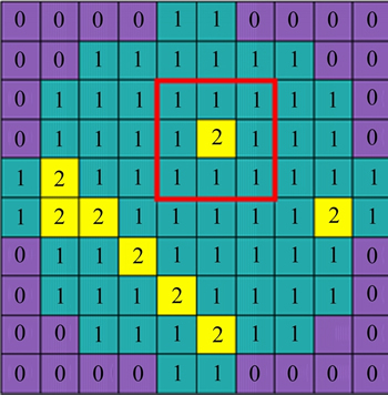
 (2)
(2) (3)
(3) is the prediction of the model; �� is applied to magnify the loss of which is small. For example, if is small, �� will magnify the loss and make the model pay more attention to the hard samples. Factor �� is employed to reduce the influence of quantity imbalance. We extend the dichotomy to the case of multiclassification. The number of parameters will increase greatly when �� is introduced in multiclassification and the influence of factor �� on the model performance is poor according to the literature [43], so we do not introduce it. The specific loss function is expressed as follows:
 (4)
(4) (5)
(5)
 (6)
(6) is the prediction result of each time, and WL is the weight parameter vector of layer L. The variance requires that input data distribute uniformly and disregard the occurrence of extreme values. When the data distribution is multipeak, the ability to describe the uncertainty is reduced. The essence of information entropy is to describe the degree of confusion, which can also be interpreted as uncertainty. We further use entropy to represent the uncertainty of the model, the expression is shown in formula (7), where p is the probability distribution of T sampling results, and I is the number of categories. The decision result is the category with the highest probability during sampling.
 (7)
(7)
 (8)
(8) (9)
(9) (10)
(10)