J. Cent. South Univ. (2016) 23: 604-622

DOI: 10.1007/s11771-016-3107-z

Time-domain compressive dictionary of attributed scattering center model for sparse representation

ZHONG Jin-rong(钟金荣), WEN Gong-jian(文贡坚)

Science and Technology on Automatic Target Recognition Laboratory, National University of Defense Technology, Changsha 410073, China

 Central South University Press and Springer-Verlag Berlin Heidelberg 2016

Abstract: Parameter estimation of the attributed scattering center (ASC) model is significant for automatic target recognition (ATR). Sparse representation based parameter estimation methods have developed rapidly. Construction of the separable dictionary is a key issue for sparse representation technology. A compressive time-domain dictionary (TD) for ASC model is presented. Two-dimensional frequency domain responses of the ASC are produced and transformed into the time domain. Then these time domain responses are cutoff and stacked into vectors. These vectored time-domain responses are amalgamated to form the TD. Compared with the traditional frequency-domain dictionary (FD), the TD is a matrix that is quite spare and can markedly reduce the data size of the dictionary. Based on the basic TD construction method, we present four extended TD construction methods, which are available for different applications. In the experiments, the performance of the TD, including the basic model and the extended models, has been firstly analyzed in comparison with the FD. Secondly, an example of parameter estimation from SAR synthetic aperture radar (SAR) measurements of a target collected in an anechoic room is exhibited. Finally, a sparse image reconstruction example is from two apart apertures. Experimental results demonstrate the effectiveness and efficiency of the proposed TD.

Key words: attributed scattering center model; parameter estimation; dictionary; time domain

1 Introduction

The target model generation, consisting of the scattering center extraction and the parameter estimation, from synthetic aperture radar (SAR) images is significant for automatic target recognition (ATR) [1-3] systems. For generating an attributed scattering center (ASC) model of target, Gerry et al [4] proposed a maximum- likelihood based estimation method. Koets and MOSES [5] and Akyildiz [6] developed this method. Maximum-likelihood methods must solve a no-line, no-convex minimization problem.

In recent years, sparse representation technology develops rapidly, and parameter estimation technology based on sparse representation has been proposed [7-13]. Sparse representation based methods transform the parameter estimation problem into a signal component selection problem by sampling the parameter space [14-18]. It accomplishes order selection and parameter estimation at the same time. It is indicated that the estimation error of sparse representation variance can approximate the Cramér-Rao bound (CRB) [7, 11-13].

There are many sparse representation based estimation works [7-12] on ideal-point scattering center model or 2D-GTD scattering center model, but few sparse representation based methods [13] for ASC parameter estimation. The reason may be that the complicated ASC model will result in a huge andunmanageable dictionary. Existing sparse representation based estimation methods [7-13] construct separable dictionaries in the frequency domain. We found the energy of response of ASC model concentrating on small regions in the time domain. We proposed a time-domain type of dictionary for ASC sparse representation, exploiting such a characteristic to reduce the data size of the dictionary. This kind of time-domain dictionary (TD) is applicable for several applications, such as parameter estimation, feature extraction, sparse imaging, data compression and compressive sensing.

The construction method of TD can be sketched as follows: calculate 2-D frequency responses of the ASC model and transform them into the time domain, cut off the low-energy area of the time domain responses and use them to build the TD. Compared with the FD, the TD is a quite sparse matrix; most elements of it are zero. So, it can be compressed into small data size and remarkably reduce recourse costs. This paper is organized as follows: First, the detailed construction method is presented.Then several extendable TD models are listed and explained. In the experiments, the performance of the TD is analyzed. In addition, we use the TD to estimate ASC parameters from an anechoic-chamber collected SAR image to demonstrate its effectiveness.

The contributions of this paper are as follows. First, a novel conception of time-domain compressive dictionary for sparse representation of SAR data is proposed. It is of generalization for radar signals of man-made targets. Second, a typical construction method of TD is presented. It is helpful for data size reduction. Third, four types of extended TD and their construction methods are proposed for some common applications.

2 Signal model

Though multi-polarization is significant research field [19-20], we study single polarization only in this work because our TD and the construction method of TD are independent of the polarization. An SAR image in the frequency-crossrange domain is a 2-D matrix  where Mf and Mp are column number and row number.  is the scattering response of target;  is noise. In the high-frequency region, can be approximated by a sum of P individual scattering center terms  So, the signal model is

                (1)

where  is the parameter set of the P scattering centers, and  is the parametric model of one scattering center. The ASC model [4] is

     (2)

where f _c is the center frequency and c is the velocity of light. In a parameter set of one scattering center  A_i is the amplitude; x_i, y_i indicate the location (i.e., cross range and range, respectively); α_i is a frequency-dependent factor; L_i is the length of the scattering center;  is the direction angle; and γ_i is the dependence factor on f. When  it is a local scattering center; when γ_i=0, it is a distributed scattering center.

Stack  into vector  where   is the m-th sample coordinate of  in the frequency-crossrange.is the measurement manifold. Vector  and  into vector   and  respectively, then the experession (1) can be rewritten in vector form of  and

3 Dictionary-based parameter estimation

Suppose that  is a six-dimensional space expanded by parameters   are P points in  A_i, i=1, …, P can be viewed as amplitudes of these points. is sparse on such a parameter space  We mesh the continuous space  into a grid,  Here, N is the number of grid points. The coordinate of a grid points is  Use the signal component of  to construct a dictionary  The measurement data are a superposition of these components,

                                      (3)

where is a sparse vector, of which only a few elements are nonzero. The parameter estimation problem has been transformed into a signal component selection problem. The parameters can be obtained by solving a l₀-regulated optimization [14-18],

                 (4)

The number of nonzero elements,  is the model order. Suppose that the nonzero elements are  k=1, …, P. The attributed  of  is the parameters  and amplitude  Traditional dictionaries for SAR images are constructed in the frequency domain. Denote  and  can be expressed as

 (5)

where  is an FD, which also can be expressed as a matrix consisting of column vectors,  

4 Time-domain dictionary

As shown in Fig. 1, the amplitudes of the responses of ASC model are well distributed in the frequency domain while they uneven distribute in the time domain. In another words, the energy concentrates on several small regions in the time domain. This characteristic do not depend on the measurement SAR data, but a natural characteristic of the ASC model. We exploit it to build a compressive TD that is a spare matrix.

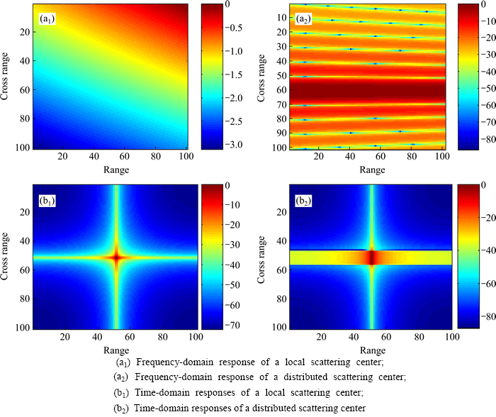
Fig. 1 Frequency/time domain responses of ASC model:

4.1 Basic method

For  a grid point in  let  and calculate 2-D frequency domain responses  by Eq. (2)

         (6)

Transform  to the time domain:

                                        (7)

where  represents the 2-D inverse fast Fourier transform (IFFT). Stack  into a  vector:

                                 (8)

where  Check each element of  and set the elements smaller than threshold  to zero:

                       (9)

where  is an adaptive threshold determined by  and a preset threshold β_d (β_d<0) of the entire dictionary.

                         (10)

Get  for all  n=1, …, N. TD  is given by

                                (11)

Based on  we establish a time-domain sparse representation model. Transform the SAR frequency domain data  to the time domain:  Stack it into  vector d. The time-domain sparse representation model is expressed as

                                     (12)

Solve model (12) and interpret the sparse vector  to obtain  the parameter set of the ASCs:

                 (13)

Taking noise into consideration, s_n is deemed as zero elements:   is a preset threshold according to the noise level. The larger the β_d is the more the elements are zero. TD becomes a quitesparse matrix, which is helpful for data size reduction. TD is not locked to a particular solution method; TD can be applied to almost all of the common sparse representation models for radar signals. In addition, as a spare matrix, TD may be beneficial to reducing the burden of computation. Although we did not attempt to prove this, it is theoretically tenable.

4.2 Procedures

The TD is obtained in two steps: sampling and calculation.

Step 1: Sample the continuous parameter space  into discrete space  Since the distributed SC and local SC are mutually exclusive, either  or  must occur. Therefore, parameter space  consists of a local scattering center’s parameter subspace  and a distributed scattering center parameter of subspace  α takes  discrete values, [-1, -1/2, 0, 1/2, 1]. The other parameters x, y, γ, L,  are sampled into N_x, N_y, N_γ, N_L, and N_f points in the range of [x_a, x_b], [y_a, y_b], [γ_a, γ_b], [L_a, L_b], and  with intervals Δx, Δy, Δα, Δγ, ΔL, and  respectively. The grid number of  is with  and The grid number of  is   with  The total number of grids of  is   Each coordinate  has been determined.

Step 2: Produce  for each using expressions (6)-(11), and obtain the TD of the entire parameter space

4.3 Express construction methods using operators

For convenience, we express the dictionary construction methods in the form of operators.

Definitions: F, construction operator of FD,  T, construction operator of TD,  vec, vector operator,   vec^-1, invert a vector into a 2-D matrix,  B·DB(D), interpolate the annulus sector data into equal sample rectangle data.  represents the 1D FFT and   represent the 1D IFFT. If d is a 2-D matrix, we operate on each column. Each Operator follows the distributive law.  denotes the cut off produces of formulas (9)-(10). For a 3-D matrix  where  we define

In this way, the TD construction can be expressed as

 (14)

The construction of FDcan be expressed as

          (15)

The transform between TD and FD is

        (16)

4.4 Several extendable TD models

The reason that we term our new dictionary as TD rather than an image-domain dictionary is because the image domain is just a special case of the time domain. There are several varieties of TD.

Model 1:  Interpolate, weighting with a window (such as -35 dB Tayler window), transform responses into the time domain, and cut off low-energy area. The 2-D image-domain responses of local and distributed scattering centers are shown in Fig. 2.

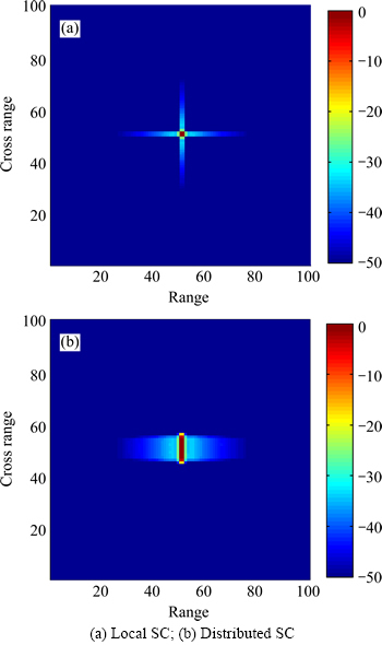
Fig. 2 2-D response of a parameter sample in extended time domain model 1:

Model 2:  Compress on range direction only, and cut off the lowenergyarea of 1-D time responses.  is a sparse matrix, but it may be denser than the matrix of Model 1. The range compressed 2-D responses of local and distributed scattering centers are shown in Fig. 3.

Model 3: If the aperture is too wide, we can divide it into a set of narrow subapertures  i=1,…, N_ap and construct a sub-TD for each subaperture.   The entire aperture is  and the measurement manifold is  The TD for the entire aperture is

Model 4: If the aperture is discontinuous, we can construct a TD for each subaperture and combine them, similar to model 3. It is very helpful in circle SAR and multiple-aspect SAR data processing. The bandwidths and apertures of subapertures can be different. Such a model can be used in the feature extraction from multi-aspect SAR data. The collection geometries of model 3 and model 4 are shown in Fig. 4.

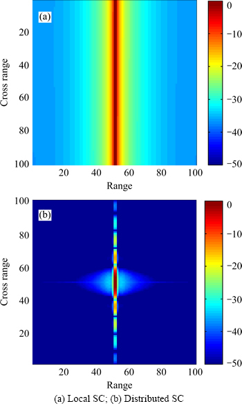
Fig. 3 2-D response of a parameter sample in extended time domain model 2:

Model 4 of TD is applicable for parameter estimation, feature extraction and sparse image reconstruction. Fourier image reconstruction method has to resample and interpolate the data into uniform rectangular grid. As there is a gap between measurement data, the interpolation will bring some error and the reconstructed image may be of low quality. The sparse imaging method can be expressed as the unified form of Eqs. (12)-(13). Let L=0,  γ=0, α=0, construct a TD only for parameter x, y. Solve model 13 to obtain amplitude A_n of very discrete position. Map all A_n to a 2-D image, or we can reconstruct the frequency-domain data and then get the image using Fourier transformation. The initial parameters of ASC model can be obtained from this image. Then, a TD of ASC model can be constructed for these sub-apertures, and re-estimate parameters of ASCs. It is feasibility to generate an ASC model from the measurement data.

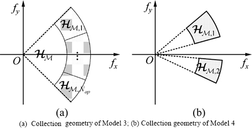
Fig. 4 Diagrams of model 3 and model 4:

5 Experimental results

The experiment consists of three parts: First, indexes λ,  and ρ are verse the cutoff threshold β_d. Moreover, the normal energy loss, η, brought about by cutoff processing is analyzed. Second, use TD and FD to estimate the ASC parameters from the SAR images, and then examine the parameter estimate errors and the normal error η_r and correlation μ_r of the reconstructed signals. Third, analyze the performance of the extended time domain models.

5.1 Inherent performance indexes of TD

In this section, several inherent performance indexes of TD are examined. We explain them first.

(1) Data size,  The smaller the λ, the sparser the

(2) Degradation of the maximum correlation,  The most authoritative criterion to evaluate the solution difficulty and risk of dictionaries is the restricted isometry property (RIP) [9]. Most of the time, it can be replaced by the easily calculated maximum correlation (MC) [14], denoted as  We elevate the MC degradation of the TD,

(3) Equivalence factor, ρ.  This indicates the equivalence between  and

(4) Normalized energy loss. It reflects the energy loss caused by the cut off operation in normalization.

Following, these four indexes verse β_d=[-50, -40, -30, -20] dB  are presented, in three cases. Radar parameters include start frequency f₀=8.5 GHz, stop frequency f_e=9.5 GHz, center frequency f_e=9 GHz, bandwidth B=1 GHz, interval △f=10 MHz, aperture 5°, and interval △f=0.05°. Mf=101, Mp=101, and measurement samples are M=Mf×Mf=10121. This is the row order of  and also  The range resolution and cross resolution of the SAR images is dx=c/2B= 0.15 m and dy=c/[4f_csin(f)]=0.19 m. We discretize the parameter space in three cases, which are typical in ASC parameter estimation application.

5.1.1 Case one

In this case, α=0, γ=0, L=0, the range of x is [-R/2, R/2], and the range of y is [-CR/2, CR/2], R=15 m, CR= 19 m, with interval △x=0.15 m and △y=0.19 m. The FD  is shown as an image in Fig. 5(a), while the TD  with cutoff threshold β_d=-40 dB is shown as an image in Fig. 5(b). It can be seen from Figs. 5(a) and (b) that the TD is a quite sparse matrix. The data size λ, MC degradation  normal energy loss, and equivalence factor ρ are plotted in one figure, Fig. 5(c). They are separately shown in Figs. 5(d)-(g) for convenience observation. We can see that the data size λ is reduced noticeably, at the cost of a slight degradation in  normal energy loss, and ρ. ρ is almost 1 when β_d=-50, -40, -30 dB, without a perceptible decline until β_d=-20 dB. For example, as β_d=-40 dB, λ=2.3%, and  and normal energy loss is 1.2%, ρ=0.997. It is said that the correlation between loss atom  and lossless atom  in the worst case is 0.997.

5.1.2 Case two

In this case, α=0, γ=0, x∈[-R/2, R/2] and y∈[-CR/2, CR/2], R=1 m, CR=1 m, L∈[0, 2 m], [-2°, 2°], with intervals △x=dx, △y=dy, △L=2dy, and 0.5°. The intervals are quite large, and parameter space is coarsely sampled. Our motivation for testing TD, in this case, is that: α and γ are too difficult to estimate efficiently when the location and length of the ASC do not approximate the real values. We have to obtain the location and the length first.

Test results are shown in Fig. 6. The representation of each image is similar to Fig. 5. Again, data size obviously decreases, and λ≤0.16. Energy loss and ρ deteriorate very slightly. The  is less than zero. It means that the MC does not increase but instead decreases. It is useful for parameter estimation. In this case, the intervals △x=0.15 m and △y=0.19 m are just right the image resolutions. We need to subdivide the parameter space to obtain an unbiased estimate. Next, we test the TD in such a case.

5.1.3 Case three

In this case, x∈[-R/2, R/2] and y∈[-CR/2, CR/2], R=2dx, CR=2dy, L∈[0.5 m, 1 m], [-0.5°, 0.5°], α∈{-1, -0.5, 0, 0.5, 1}, and γ∈(-10^-12, -10^-11], with intervals △x=dx/2, △y=dy/2, △L=0.1 m, △f=0.1°, and △γ=-10^-12. The intervals are small, and the sampling of parameter space is fine. Figure 7(a) shows the FD,  Figure 7(b) shows the TD  with a cutoff threshold of β_d= -40 dB.

The performance indexes versus β_d are shown in Fig. 8. Figure 8(a) depicts the indexes of  the local SC part of the TD. Figure 8(b) depicts the indexes of  In Figs. 8(c)-(f), the indexes are re-depicted separately. As with the above two cases, it can be found that the data size of the TD is much smaller than that of the FD, λ<0.1. It means that the data size decreases by 1-2 orders of magnitude. The MC increases  and normal energy loss is less than 12%. In particular, when β_d≤-30 dB, the normal energy loss is less than 4% and ρ is larger than 0.94. In particular, when β_d≤-30 dB, ρ is larger than 0.98.

As the sampling intervals of parameters become small, the intercolumn correlation of the dictionary increases. Some sparse reconstruction algorithms for highly correlated dictionaries have been developed in Ref. [7].

5.1.4 Results of four extended models

Below we examine the extended models of TD. The parameter setting is the same as case three. The model 3 and the model 4 are different in physical conception as they are suitable for different collection geometry. However, they are the same seen from the view of methodology. So, we only examine model 4, which is more general. The performance of model 3 can be inferred from the results of model 4. The settings of radar parameters for model 1 and model 2 are the same as the beginning of this section. The experiment results of model 1 and model 2 are shown in Fig. 9 and Fig. 10, respectively.

It can be seen from Fig. 9 that, the data size of the dictionary of model 1 is smaller than the standard model, while the data size of the dictionary of model 2, shown in Fig. 10, is much bigger than the standard one.

The parameter sampling setting of ASC model is the same as case three in section 5.1.3. But the radar parameter setting for model 4 is as follows. The frequency range of the first aperture is 8.5 GHz≤f≤ 9.5 GHz, and its azimuth is -2.5°≤<-0.5°. The frequency range of the second aperture is 8.5 GHz≤f≤ 9.2 GHz and its azimuth is 1°≤≤3.5°. The frequency sampling interval and azimuth sampling interval of both apertures are △f=10 MHz and △f=0.05°. There are Mf×Nf=50×50 samplings in the first aperture and Mf×Nf=51×51 samplings in the second aperture. Figure 11 shows the results of model 4. The data size ratio of model 4 is not lower than the standard one because the two apertures are smaller.

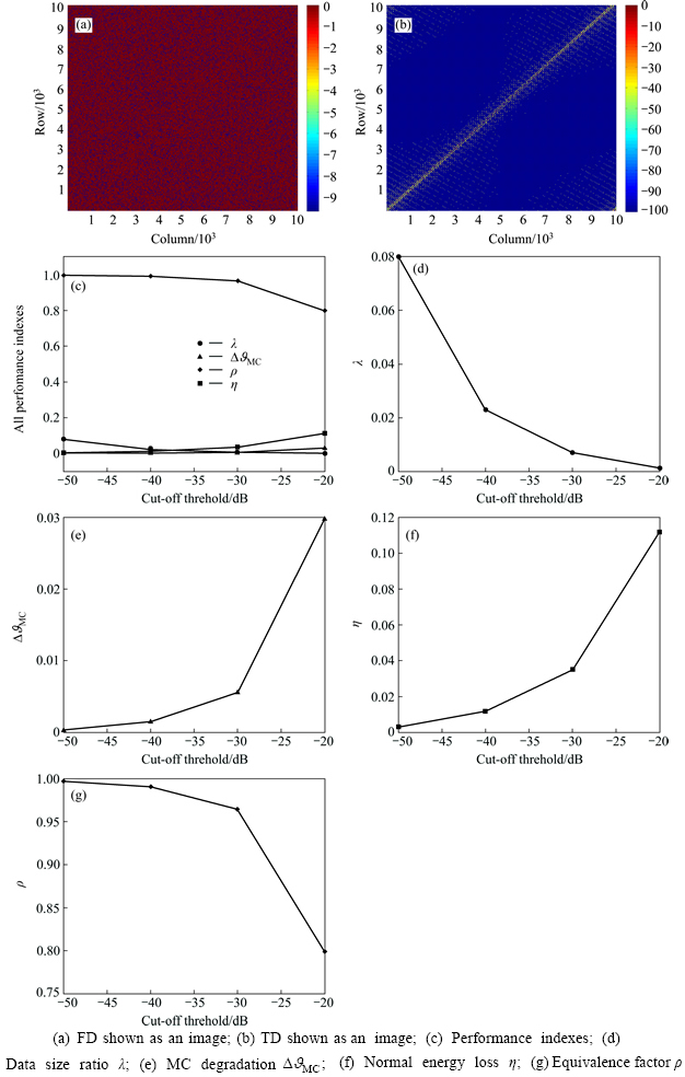
Fig. 5 Performance of TD in case one:

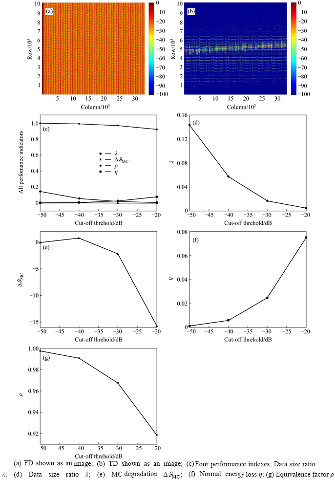
Fig. 6 Performance of coarse-parameter- sampling dictionary:

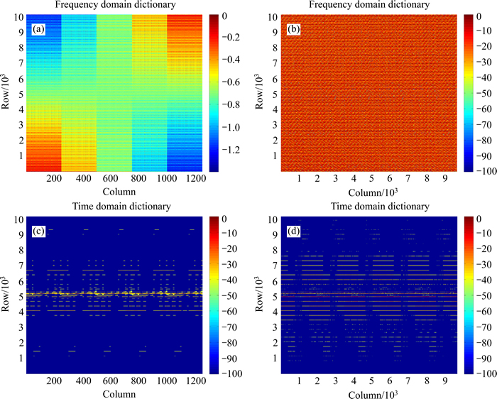
Fig. 7 FD (a, b) and TD (c, d) of fine parameter samplings, with β_d=-40 dB: (a, c) Local scattering center; (b, d) Distributed scattering center

5.2 parameter estimation

In this section, we estimate ASC parameters from SAR images using the TD and FD separately. We present the performance of the standard model of TD, which can be taken as a benchmark of the other, in comparing with the results of the FD. In addition, several performance indexes are examined, and we explain them first.

1) The straight forward evaluation approach is to examine the parameter estimation error. Use the TD and FD to estimate ASC parameters. Then we statistic the variances of parameter estimate errors and compare the variances with the CRBs. In our numerical simulation, since we know the true parameters, we carry out the experiment in this way.

2) If the true parameters are unknown, we examine the performance in this way: Get and  and reconstruct signals  or  Then, calculate the similarity, normal error η_r, and correlation μ_r between the reconstructed signals and the original signals. η_r and μ_r are defined as

It should be noted that we reconstruct both signals in frequency-domain. Next, we examine the estimation performances of the TD and FD when they are used to estimate the ASC parameters from numerical simulated SAR data and anechoic-chamber-collected SAR data. The estimation is carried out in a multistep way: Get the initial parameters from the SAR image, divide the parameter space around the initial values to construct the dictionary, and subdivide the parameter space around the last estimate result for an unbiased estimate. Subdivide the parameter space by N_Iter times, and the parameter space is  times the initial one, i_t=1, …, N_Iter. Every iteration is decomposed in two serial steps, estimating x, y, L, f first and then α, γ. Use the orthogonal matching pursuit (OMP) algorithm [17] to solve Eqs. (4) and (13).

In this section, we evaluate the parameter estimation performance of the TD using simulated data versus cutoff thresholds and signal-to-noise-ratios (SNRs). The performance of the TD is compared with the performance of FD and the CRBs. SNR is defined as the ratio of the peak image amplitude to the noise standard deviation in the image domain. It is expressed in the dB scale as follows:

                                        (17)

We form the image without any noise and determine the peak image amplitude value. Calculate  corresponding to that peak value and the desired SNR. Then, turn  into the frequency-domain noise variances

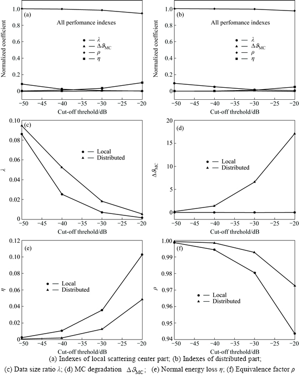
Fig. 8 Performance of fine-parameter-sampling dictionary:

5.2.1 Numerical simulation

Parameters of two SCs, S1 and S2, are listed in Table 1. S1 is local, and S2 is distributed. We simulate their scattering response. Add zero-mean white Gaussian complex noise, and form its SAR image. The cutoff threshold is  and SNR=[20, 25, 30, 35, 40]dB. For each fixed β_d and fixed SNR, carry out Monte Carlo simulation [21] 100 times. Noise is re-retaliated on every trip. The corresponding CRBsare calculated with the designated parameter values and noise.

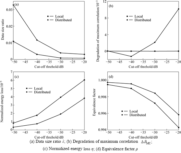
Fig. 9 Dictionary indexes of model 1:

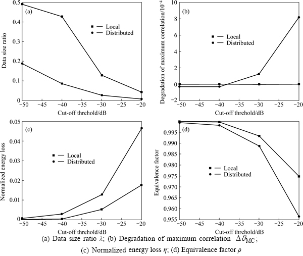
Fig. 10 Dictionary indexes of model 2:

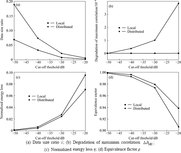
Fig. 11 Dictionary indexes of model 4:

Table 1 Parameters of two ASCs

We present the estimate variances of S1. x, y variances are in units of m². The CRBs are also shown in the same plot in Fig. 12. We can see that, when β_d=-50 dB, the variances of the TD-based algorithm are equal or very close to the estimate variances of the FD-based algorithm and CRBs. When -40 dB≤β_d≤-30 dB, all of the estimate variances, and α-detection probability Pd(α), are less accurate in different degrees. Another finding is that the lower the SNR is the estimated TD performance of x, y, and γ degrades slightly. This may occur because as signals are cut off by β_d, the noises in  are cut off covertly rather than directly. The signal loss is the same whether the SNR is low or high, but the dislodged noise is more when the SNR is low.

Similar results of the distributed scattering center S2 are presented in Fig. 13. The variances of L are in units of m², and  is in units of radians-square. We find that: 1) when β_d=-50 dB, x variances of the TD estimation are equal to the CRB, and are less accurate as β_d≥-40 dB. 2). The y and L variances of the TD estimation are very close to the CRB until β_d=-20 dB. 3) The  estimate variances keep close to the CRB for all -50 dB≤β_d≤ -20 dB. 4) When β_d=-20 dB, which is a large threshold, the x, y, and L estimate variances greatly increase. However, it should be noted that for the case of λ<0.01, the TD data size is less than 1% of the FD size. 5) An unexpected finding: The Pd(α) of the TDs are better than those of the FDs; and the larger the β_d is, the better the Pd(α) for the TDs is obtained. The reason may be that most of the noise is cut off, while most of the information remains in the main lobe. This is very useful for feature extraction in SAR ATR systems. We are more interested in the type of scattering centers rather than their precise locations and lengths. Therefore, we desire a more accurate type parameter α than an excessively pinpoint estimates of x, y, and L.

In summary, the performance of the TD is almost the same as the FD when β_d=-50 dB. They degenerate slightly in accuracy, with a remarkable decrement in data size, when β_d=-40 dB. The performance degenerates more as β_d≥-30 dB. However, it still benefits the parameter estimation since we can alter β_d in different applications.

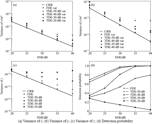
Fig. 12 Parameter estimate variances and CRB for localized scattering response with parameters {1, 1, -1, -1, 5.3×10^-12, 0, 0} versus SNR:

5.2.2 Experimental result of anechoic chamber data

We demonstrate the performance of the TD using the data of a tank model collected in an anechoic chamber. The test model is shown in Fig. 14. It is a sophisticated enough target, though it is simpler than an actual tank. Frequency f: 8.5-9.5 GHz, interval Δf=10 MHz, Mf=101; aperture =5°, interval Δf=0.05°, Mf=101, and the size of is M=Mf×Mf=10121. Add SNR=30 dB Gaussian white noise to the image shown in Fig. 11. The sparse factor is K=20.

1) An example at β_d=-40 dB.

With β_d=-40 dB, the extracted parameters by FD and TD, respectively, are listed in Table 2 and Table 3. Figure 15 shows the SAR images reconstructed from the estimated parameters. After carefully checking the results, we find that there is a frequency-dependence factor of S18 and a slight amplitude deference between the parameters extracted by TD and parameters extracted by FD. The other parameters are almost the same. Subdivide the parameter space N_Iter=10 times. The data size is λ=5.46% on average.

2) Statistics results.

The experimental procedure is as follows: For a fixed β_d, we add zero-mean white Gaussian complex noise to make SNR=30 dB. We then obtain the parameter estimations using both the FD- and TD-based parameter estimation algorithms. We repeat this process for 30 different images with 30 different random noise realizations. Since we do not know the true parameter values, we investigate the mean reconstruction error η_r and correlation μ_r of the TD and FD. The statistical data is obtained separately at cutoff threshold β_d=[-50, -40, -30, -20]dB. The results are shown in Fig. 16. We see that reconstructed signals exhibit small differences. If our purpose and task is to obtain a presentation of sparse the SAR image, we can make a judgment that the TD and FD are practically equivalent. If our purpose is to obtain the parameters, the result in Fig. 16 can, in a manner, demonstrate that the differences between TD-estimated parameters and FD-estimated parameters are very small.

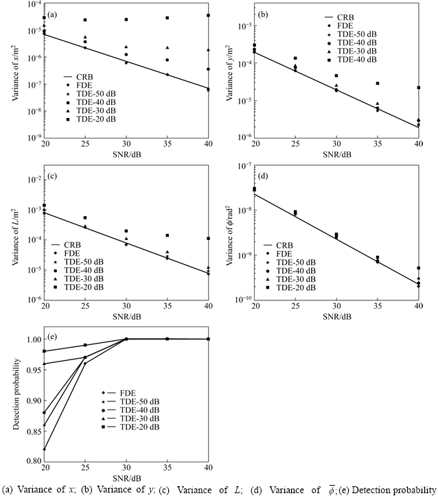
Fig. 13 Parameter estimate variances and CRBs for distributed scattering response with parameters {10, 0, 1, 1, 0, 2, 0.5} versus SNR:

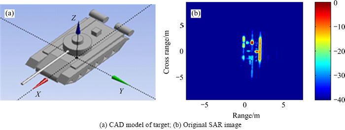
Fig. 14 Data collected in anechoic chamber:

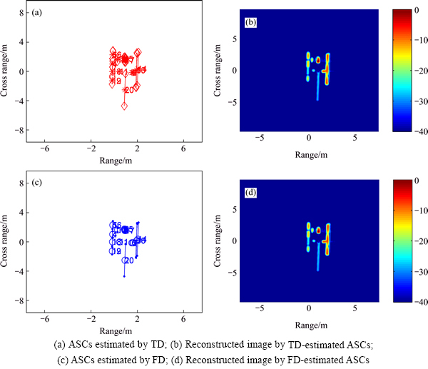
Fig. 15 Estimated ASC parameters and images reconstructed by parameters:

Table 2 Estimated parameters of complex target by FD

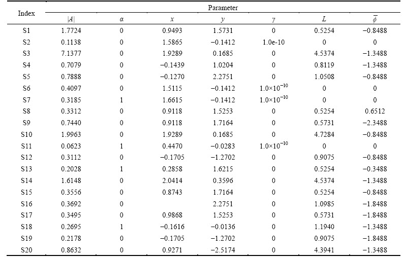
Table 3 Estimated parameters of complex target by TD

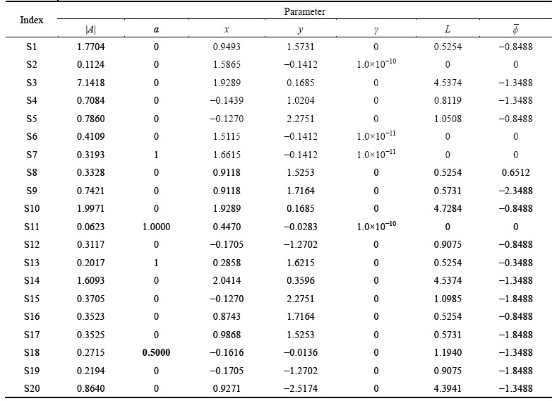
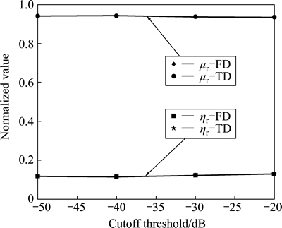
Fig. 16 Statistics result of estimation performance of both TD and FD

5.2.3 sparse representation based imaging from SAR data with gap

One of the key utilities of parameter estimation technology, or sparse representation technology, is to reconstruct SAR image from SAR data with hiatus. In this example, we present the parameter estimation performance of TD as the two aspects are separated. It matches Model 4. The frequency range of the first aperture is 8.5 GHz≤f<9 GHz, its azimuth is -2.5°≤<0°. The frequency range of the second aperture is 9 GHz≤f<9.5 GHz, its azimuth is 0°≤<2.5°. The frequency sampling interval and azimuth sampling interval of both apertures are △f=10 MHz and Δf=0.05°. There are Mf×Nf=50×50 samplings in the first aperture and Mf×Nf=51×51 samplings in the second aperture. The original frequency-domain data are shown in Fig. 17(a).

We present image reconstructions from the two apertures using standard Fourier method. The reconstructed images from the first aperture and the second aperture are shown in Figs. 17(b) and (c). It can be seen that the structure of target is highly smoothed and unclear due to the low resolution. Then we synthesize the two apertures as one, and carry out Fourier-based image reconstruction to it. The reconstructed image is shown in Fig. 17(d), in which obvious lobes arise. the reconstructed image is of poor quality. Due to the high image sidelobes, the structure of the target is highly distorted.

Below it will be shown that the image quality can be improved through a method consisting of a parameter estimation and a signal reconstruction. The purpose of estimating the parameters is to reconstruct SAR data and images. So, this processing can be viewed as sparse representation. We achieve the parameter estimation using our TD. The estimation method of the scattering center model is in two steps.

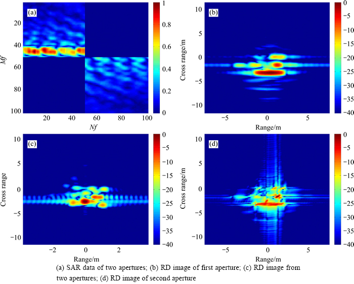
Fig. 17 Original SAR data with gap and images:

In the first step, a TD is constructed with following parameter sampling setting. α=0, γ=0, L=0, the range of x is R=8 m and the range of y is CR=10 m, interval Δx= 0.1 m and Δy=0.1 m. Such setting is similar to the case one presented in section 5.1.1. we use this dictionary to estimate the amplitude of all scattering centers from the notched SAR data, and solve the model (13) by l₁-regularized algorithm [22-23]. The sparse parameter lambda=0.02 is selected manually. The result is a sparse representation of the target consisting of scattering centers. Once the sparse representation is obtained from the two apertures, it is possible to generate signatures at nearby angles and nearby frequencies. Figure 18(a) shows the reconstructed SAR data. The image formatted from this reconstructed data by Fourier method is shown in Fig. 18(b). As can be seen from Fig. 18(b), the image resolution is more better than Figs. 17(b)-(d). From this SAR image, initial parameters of ASCs are obtained. In this step, the extraction method models all scattering phenomena using local scattering centers. It gives a faithful reconstruction of the data.

In the second step, though we can use the method presented in section 5.2.1 to select order and estimate parameters of ASC model, we present a simpler algorithm for the application of image formation. We take a algorithm called CLEAN to extracting the ASC model from the reconstructed image shown in Fig. 18(b). It iteratively estimates the next-largest scattering center and removes the prediction from the observed data. Firstly, find the peak of the image and segment the region of it using the watershed segmentation technology [5]. The threshold for image segmentation is -30 dB. Secondly, one TD is constructed for every region, with the same parameter sampling setting as the case three in section 5.1.3. Then we estimate parameters by OMP algorithm as in section 5.2.2. The iteration number is chosen n_iter=3. After each estimation of one scattering center, subtraction of the estimated signal yields a new set of observations. Repeat the segmentation and parameter estimation until a desired number of scattering centers are extracted, or the residual energy is below a desired level. In this example the maximum number of scattering centers (sparse parameter) is K=20 and the desired level of residual energy is ζ=0.01. Resembling to step one, the result in this step, an ASC model extracted from the observed data is another sparse representation of target. The sparser ASC representation is a more efficient means of modeling the non-point-scattering phenomenon. Since the ASC model is faithful [4], it gives a more accurate reconstruction of the data. Figure 18(c) shows the reconstructed data from the ASC representation, while Fig. 18(d) displays the image reconstruction from it using Fourier transformation. The reconstructed SAR image is of better quality than the original images in Figs. 17(b)-(d). It can be seen that features in the sparse reconstruction Fig. 18(d) are well-resolved.

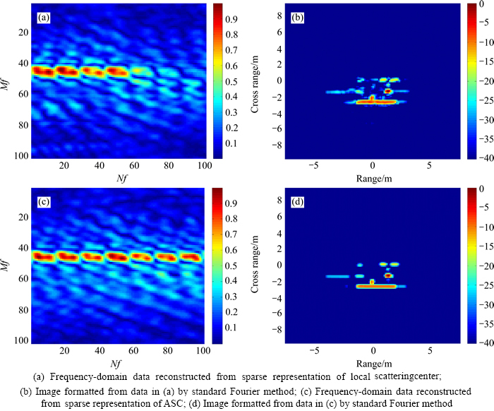
Fig. 18 Reconstructed SAR data and images:

6 Conclusions

a kind of sparse representation dictionary called time-domain dictionary (TD) for ASC model parameter estimation is developed. Such a dictionary consists of cutoff time-domain responses. It makes the TD to be a sparse matrix which can be compressed in a smaller data size than its original size. The data size of dictionary remarkably reduces at a negligible cost of accuracy degeneration. Compared with a traditional FD, its data size is reduced by 1-2 orders. Both numerical and anechoic-room data experiment results in several applications have demonstrated that the TD-based methods can obtain accurate ASC parameter estimations from SAR measurements. Another advantage of the compressive TD is that it does not require special producing and solving algorithm. Therefore, most of the existing dictionary-based methods for SAR images can employ the TD to save resources. Extending the TD to a 3-D canonical shape-scattering model [24] is the further research.

References

[1] POTTER L C, CHIANG D M, CARRIERE R, MICHAEL J G. A GTD-based parametric model for radar scattering [J]. IEEE Transactions on Antennas and Propagation, 1995, 43(11): 1058-1067.

[2] POTTER L C, MOSES R L. Attributed scattering centers for SAR ATR [J]. IEEE Transactions on Image Processing, 1997, 6(1): 79-91.

[3] DUNGAN K, POTTER L C. 3-D imaging of vehicles using wide aperture radar [J]. IEEE Transactions on Aerospace and Electronic Systems, 2011, 47(1): 187-200.

[4] GERRY M J, POTTER L C, GUPTA I J, MERWE A. A parametric model for synthetic aperture radar measurements [J]. IEEE Transactions on Antennas and Propagation, 1999, 6(1): 1179-1188.

[5] KOETS M A, MOSES R L. Feature extraction using attributed scattering center models on SAR image [C]// EDMUND G Z. Proceeding in Algorithms for Synthetic Aperture Radar Imagery VI. Orlando: SPIE, 1999, 3721: 104-115.

[6] AKYILDIZ Y. Feature extraction from synthetic aperture radar imagery [D]. Ohio, USA: Dept Electron Eng, Ohio State University, 2000.

[7] AUSTIN C D. Sparse methods for model estimation with applications to radar imaging [D]. Columbus: The Ohio State University, 2012.

[8] YANG Z Y, XING Y, XIE S L, DING S X. Nonnegative blind source separation by sparse component analysis based on determinant measure [J]. IEEE Transactions on Neural Networks and Learning Systems, 2012, 23(10): 1601-1610.

[9] DONOHO D L. Compressed sensing [J]. IEEE Transactions on Information Theory, 2006, 52(4): 1289-1306.

[10] DU Xiao-Yong, HU Wei-Dong, YU Wen-Xian. Parameter estimation of GTD model based on sparse component analysis [J]. Journal of Electronics & Information Technology, 2006, 28(2): 363-366. (in chinese)

[11] ZHAN Rong-hui, HU Jie-min, ZHANG Jun. A novel method for parametric estimation of 2D geometrical theory of diffraction model based on compressed sensing [J]. Journal of Electronics & Information Technology, 2013, 28(2): 419-425. (in chinese)

[12] AUSTIN C D, ERTIN E, MOSES R L. Sparse signal methods for 3D radar imaging [J].IEEE Journal of Selected Topics in Signal Processing, 2011, 5(3): 408-423.

[13] LI Fei, JIU Bo, LIU Hong-wei. Sparse representation based algorithm for estimation of attributed scattering center parameter on SAR imagery [J]. Journal of Electronics & Information Technology, 2014, 36(4): 931-937. (in chinese)

[14] DONOHO D L, ELAK M, TEMLYAKOV V N. Stable recovery of sparse over complete representation in the presence of noise [J]. IEEE Transactions Information Theory, 2006, 52(1): 6-18.

[15] CADES E, ROMBERG J, TAO T. Stable signal recovery from incomplete and inaccurate measurements [J]. Comm Pure Appl Math, 2006, 59(8): 1207-1223.

[16] CEVHER V, KRAUSE A. Greedy dictionary selection for sparse representation [J]. IEEE Journal of Selected Topics in Signal Processing, 2011, 5(5): 979-988.

[17] TROPP J A, GILBERT A C. Signal recovery from random measurements via orthogonal matching pursuit [J]. IEEE Transactions on Information Theory, 2007, 53(12): 4655-4666.

[18] SELESNIC I W, BAYRAM I. Sparse signal estimation by maximally sparse convex optimization [J]. IEEE Transactions on Signal Processing, 2014, 59(11): 5202-5211.

[19] DAI Huan-yao, WANG Xue-song, LI Yong-zheng. A new polarimetric method by using spatial polarization characteristics of scanning antenna [J]. Transactions on Antennas and Propagation, 2012, 60(3): 1653-1656.

[20] QIU Wei, ZHAO Hong-zhong, ZHOU Jian-xiong, FU Qiang. High-resolution fully polarimetric ISAR imaging based on compressive sensing [J]. IEEE Transactions on Geoscience and Remote Sensing, 2014, 52(10): 6119-6131.

[21] KAY S M. Fundamentals of statistical signal processing volume I: estimation theory [M]. New Jersey: Prentice Hall Pearson Education, 1993: 157-214.

[22] KIM S J, KOH K, LUSTING M, BOYD S, GORINEVSKY D. A method for large-scale l1-regularized least squares [J]. IEEE Journal on Selected Topics in Signal Processing, 2007, 1(4): 606-617.

[23] Simple matlab solver for 11-regularized least squares problems. [2014-06]. http://web.stanford.edu/~boyd/l1_ls/.

[24] JACKSON J A, RIGLING B D, MOSES R L. Canonical scattering feature models for 3D and bistatic SAR [J]. IEEE Transactions on Aerospace and Electronic Systems, 2010, 46(2): 525-541.

(Edited by YANG Hua)

Foundation item: Project(NCET-11-0866) supported by Education Ministry's new Century Excellent Talents Supporting Plan, China

Received date: 2015-01-12; Accepted date: 2015-09-23

Corresponding author: ZHONG Jin-rong, PhD Candidate; Tel: +86-18670019557; E-mail: zhong_nudt@163.com