ARTICLE

J. Cent. South Univ. (2019) 26: 2281-2294

DOI: https://doi.org/10.1007/s11771-019-4173-9

Hybrid ToA and IMU indoor localization system by various algorithms

CHEN Xue-chen(陈雪晨)¹,CHU Sheng(楚盛)¹, LI Fan(李繁)¹, CHU Guang(楚广)²

1. School of Electronics and Information Technology, Sun Yat-Sen University, Guangzhou 510275, China;

2. School of Metallurgy and Environment, Central South University, Changsha 410083, China

Central South University Press and Springer-Verlag GmbH Germany, part of Springer Nature 2019

Abstract: In this paper, we integrate inertial navigation system (INS) with wireless sensor network (WSN) to enhance the accuracy of indoor localization. Inertial measurement unit (IMU), the core of the INS, measures the accelerated and angular rotated speed of moving objects. Meanwhile, the ranges from the object to beacons, which are sensor nodes with known coordinates, are collected by time of arrival (ToA) approach. These messages are simultaneously collected and transmitted to the terminal. At the terminal, we set up the state transition models and observation models. According to them, several recursive Bayesian algorithms are applied to producing position estimations. As shown in the experiments, all of three algorithms do not require constant moving speed and perform better than standalone ToA system or standalone IMU system. And within them, two algorithms can be applied for the tracking on any path which is not restricted by the requirement that the trajectory between the positions at two consecutive time steps is a straight line.

Key words: indoor localization; time of arrival (ToA); inertial measurement unit (IMU); Bayesian filter; extended Kalman filter; MAP algorithm

Cite this article as: CHEN Xue-chen,CHU Sheng, LI Fan, CHU Guang. Hybrid ToA and IMU indoor localization system by various algorithms [J]. Journal of Central South University, 2019, 26(8): 2281-2294. DOI: https://doi.org/10.1007/s11771-019-4173-9.

1 Introduction

In recent years, designing an effective indoor positioning system (IPS) [1, 2] becomes more and more popular thanks to the rapid development of wireless technologies and proliferation of mobile computing devices. IPS dominates in substantial applications around the world. To name a few, one can consider the orientation of firefighters at the fire area, location detection of customers after they enter a shopping mall to guide them to the areas that they need and find tagged searching robots in a disaster scene. The positioning information can help the ad-hoc network to improve the ability of self- organizing as well.

The well-known global positioning system (GPS) can provide navigation capability to various devices by adding GPS accessories to them. However, because of the presence of non line of sight (NLOS) transmission between satellites and receivers inside, GPS-based system is not applicable. And considering about the cost constraint, GPS is not a good choice for indoor localization as well. Without the use of GPS, a great number of solutions are proposed to solve the problem. Among them, wireless sensor networks (WSN) are adopted more and more frequently to render efficient indoor positioning services, due to their property of low cost and wide coverage. Positioning approaches by WSN is capable to be divided into two types: range based and range free.

Range based systems: Compared to range free systems, these systems exhibit higher accuracy. They utilize the range measurements between the moving node and an array of anchor nodes at known locations to assist the positioning. The range is calculated using various methods including time of arrival (ToA) [3], time variance of arrival (TDoA) [4], received signal strength indication (RSSI) [5, 6], angle of arrival (AoA) [7] and etc. Within them, by ToA way, range survey is achieved by controlling the signal transmission time with light velocity. As a result, concerning two- dimensional location, uncertain nodes are supposed to be on a circle centered at the related anchor nodes provided by ToA. Then triangulation algorithm or maximum likelihood estimator (MLE) is applied to clarifying the location of the uncertain nodes. Therefore, the system demands at least three anchor nodes.

Range free systems: These systems include distance based localization system and proximity based localization system. The former one calculates the distance between the moving node and anchor nodes, then localizes the position of the object. Different from range based methods, the distance is calculated approximately through multiplying hop number from the anchor node to moving node by average distance of each hop. The typical distance based schemes include DV-hop, Amorphous and etc [7-9]. The latter one provides only coarse location (perhaps the nearest room) instead of providing coordinate location. Examples include RFID and bluetooth systems.

Automobile guidance, navigation in ship or missiles and other applications substantially employ inertial navigation system. It is generally composed of accelerometers and gyroscopes. The former determines accelerated and the later determines angular rotated speed. We compute the top angles and speed through dead reckoning approach with the help of collected data. Then, we easily attain the estimated locations. Lately, due to the fact that the increasing mobile computing devices are equipped with inertial sensors and DR methods become increasingly practical for indoor navigation. In Refs. [10-14], the authors introduced INS into IPS design. These methods rely on inertial sensors to render pedestrian dead reckoning (PDR) solutions. On the other hand, because of noisy inertial sensors estimating, INS generally tends to gather error over the time and distance. As a result, various techniques have been introduced to correct the tracking error of a DR system. A ranging sub-system was developed with infrastructure to constrain and correct the error of DR sub-system [11]. However, the infrastructure needs to be a sparse one. In Refs. [12, 13], authors proposed to integrate PDR system with RSS information obtained by RFID tags and IEEE 802.15.4a anchors respectively. Though the system could obtain accurate positioning estimates in particular environment, the performance would deteriorate if the RSS fluctuation is serious. In Ref. [14, 15], authors presented hybrid system that consists of fingerprint method and DR solution with the aid of a particle filter. However, the positioning could be imprecise due to the unstable property of fingerprint method.

In this paper, we introduce to combine WSN with INS, working out inside positioning issue. Firstly, we apply ToA approach to WSN because of relatively high accuracy and low complexity of computation. Inertial measurement unit (IMU) dominates the INS. Hence, we apply hybrid scheme. The integration of these two schemes is capable to achieve error recovery. Moreover, the accuracies of standalone systems are significantly facilitated. Sometimes, the communication of three anchors for ToA scheme is difficult to mask. Obviously, even if there are only two anchors, the estimate accuracy of a mixed method is better than that of the ToA scheme due to the hybrid scheme. In Ref. [16], we introduced to integrate two methods. Meanwhile, they employ extended Kalman filter (EKF), estimating pedestrian location. Therein TDoA approach is applied, clarifying the ranges in WSN. However, it is significantly more complicated than ToA method. Apart from that, the author supposed that the object maintains uniform motion. But, the pure uniform motion is absolutely impossible around the real world particularly for non- pedestrian navigation scheme. The hybrid method was studied [17]. It combined DR and RSSI, applying EKF to correct the navigation error by DR in real-time. They proposed an adaptive step length algorithm and introduced it to estimate the moving distance between two time steps. Hence, the trajectory between two consecutive time steps needs to be a straight line. Different from above work, our contribution is shown below:

1) Here are three hybrid approaches, EKF, PF and MAP. We consider posterior probability for this sequential procedure. As shown in simulation results, the performance of hybrid ToA and IMU is splendid on utter ToA so as to DR method. Even though the measurement model only possesses two anchors, one of the methods can still beat standalone ToA scheme. Meanwhile, the rest ones still have better performance than pure DR scheme.

2) If the EKF or PF hybrid method is adopted, there is no need to restrict the motion path or motion characteristics because the acceleration and angular velocity information construct the model for transiting, rather than artificial step estimation. When the requirement that the trajectory between the positions at two consecutive time steps is a straight line is satisfied, similar to the case in Refs. [16, 17], hybrid method with MAP can be applied. And experimental results show that if only two anchors are adopted in observation model, MAP algorithm has the best performance among three kinds of hybrid methods. In the other hand, though the moving path is restricted by the requirement illustrated as above, the characteristics of movement is not restricted for MAP algorithm, that is, different from the work in Refs. [16, 17], the tracking object can move with non-constant speed due to the same reason that while modeling the transition of the process, acceleration and angular rates obtained from IMU are used, not the pedestrian steps.

The following content of the paper is shown below. In Section 2, it illustrates the achievement of the whole hybrid scheme. As for Section 3, three valuation algorithms are proposed. In Section 4, we display superior performance of algorithms by simulation consequences. Lastly, we conclude with a brief discussion of future work in Section 5.

The notation used in this letter is according to the convention. Symbols for matrices (upper case) and vectors (lower case) are in boldface. The material in this paper was presented in part in Ref. [18].

2 System overview

Generally, capture system and processing terminal are two most vital parts of our model, as shown in Figure 1. With help of known position, the information, inertial measurement is capable to be corrected by the model, from the shifting object to anchors. The range measurement also needs to be corrected.

Inertial information: IMU380ZA-409 provided by MEMSIC, is applied to acquiring inertial information. A 9-DoF inertial board dominates in the IMU380ZA-409. It contains three axes of angular rate sensing, linear acceleration sensing. Moreover, three axes of magnetometer are selectable, supplying nine degrees of inertial measurements. Figure 2 displays the change from the partial coordinate frame of IMU of shifting target to the reference coordinate system in 2D scenario. x_l-axis, y_l-axis and z_l-axis constitute local coordinate system while x_r-axis, y_r-axis and z_r-axis constitute reference coordinate system. The angular rate sensors obtain the angular rotation rates around the corresponding axes in the local coordinate system. We determine the orientation of positive rotation according to the left hand rule. For instance, zero angular rates are acquired from the x_l and y_l direction as the IMU380ZA is on a level, rotating clockwise. Meanwhile, the sensor on z_l direction is expected to obtain a positive angular rate. More details were illustrated in Ref. [19].

Figure 1 Flowchart of overall system

Figure 2 Transition from local coordinate frame to reference coordinate frame

The IMU component can hardly link processing terminal wirelessly. Hence, the zigbee component DRF1605H provided by DTK Electronics is apply to completing wireless communication. DRF1605H links the IMU380Za-409 via TX/RX pin. Moreover, it transforms UART for fitting Zigbee wireless network. Lastly, the component DRF2618A, receiving data from Zigbee, sends information to terminal module with USB.

Range measurements: We use the MCS410CA of the cricket provided by MEMSIC to get the range measurements by ToA method. The object in motion also carries a cricket mote which persistently deliveries consistent radio frequency (RF) and ultrasound pulses. They will be accepted at known positions by other cricket motes immobilized to other nodes, which get range measurements by creating different arrival times between signals. The information is then sent to MIB510. Data will be transmitted to the terminal via USB.

The actual equipment includes two parts: capture and rece4iver. The capture system, which includes IMU380ZA-409, DRF1605H and one cricket mote, in which the black cable charges DRF1605H via the mobile power supply below the receiver for processing terminal includes DRF2618A and wireless gateway MIB510.

At the terminal, the output rate of IMU data is configurable. Taking an instance, the output period will be 0.1 s if the rate is equal to 10 Hz. Then, a triple (a_xl, a_yl, ω_zl) is taken down at every 0.1 s. a_xl, a_yl represent speed-up values on x_land y_l direction respectively. ω_zl represents the angular rate around z_l and two dimensional situation. The direction cosine matrix shown below is capable to acquire the speed-up values a_xr, a_yr along x_r- and y_r-axis.

                 (1)

where represents the angle between the local coordinate system and the reference coordinate system now, which is also the heading angle that researches are expected to describe below.

As shown in following sections shown, △t indicates the output cycle of IMU. Moreover, we ignore r in x_r, y_r and z_r for the sake of simplicity.

3 Algorithms

It is dynamic issue for orienting mobile target. Here are two models for analysis: the system and observation model. The former represents the unfolding of time state. On the other hand, the latter depicts the state corresponding with noisy inspection. Then, three kinds of algorithms will be introduced to tackle the navigation issue. And we tend to apply the fusion of inertial measurements and range measurements. The recursive Bayesian method covers all three methods. Specifically, posterior probability density function of states is vital to fulfill estimation. Next, we define the state vector as s_k at the k-th time interval. And we define the measurement vector as z_k, where…, K} and K is the total number of time steps.

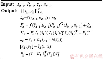
3.1 Extended Kalman filter algorithm

The Kalman filter was displayed in Ref. [20]. It applies several of noisy measurements over time, introducing state estimations. The estimate result is calculated through mean squared error minimum. Moreover, state shift and observation formula are essential to the computation. In Ref. [21], a sub- optimal Bayesian filter was proposed known as the extended Kalman filter, concerning nonlinear problems. The state shift formula and measurement formula of EKF are represented as follows,

                      (2)

where u_k-1 is the control sequence at the (k-1)-th time interval;is a nonlinear formula. The equation shifts the state at time step k-1 to k. And describes the nonlinear formula, mapping s_k to z_k. Apart from this, n_s, n_z and n_u are dimensions of the state, measurement and control vectors, respectively. ω_k and v_k describe the shift and measurement noises. These two noises are initialized to 0 mean multivariate Gaussian noises with covariance matrix Q_k and R_k.

Concerning the situation, five state variables are under consideration. Specifically, s_k is shown as follows:

                        (3)

Herein, x_k and y_k respectively denote the x- and y-coordinate values of the position in the reference coordinate frame at the k-th time interval, v_x,k denotes the speed of target in x orientation while v_y,k in y direction at the k-th time interval. φ_k denotes the heading angle at the k-th time interval.

We suppose n samples, outputting from IMU between time step k-1 and time step k. Within them, the i-th sample is (a_xl,i, a_yl,i, ω_z,i). In the sequel, φ_i=φ_i-1+Δφ_i=φ_i-1+ω_z,iΔt. And Eq. (1) achieves the computation of a_x,i, a_y,i. In the next 4 paragraphs, we initiate the analysis of state shift.

First, the shift distance between time step k-1 and k in x orientation can be represented as:

The same derivation can be applied for computing the distance in y orientation,

The speeds of state shift are built as follows,

The heading angle shifting from k-1 to k is described as

Overall, the state shift formula f(s_k-1) is linear,

Under renewal stage, shift formula firstly achieves renewal with the help of the measurement formula. For ideal situation, it is supposed to be pulled back to the right position when the consequence from the dead reckoning drifts apart. Hence, we describe the nonlinear problem by the following equation:

Suppose that m anchor nodes exit. represents the distance between the ith anchor node and the mobile one and (xⁱ, yⁱ) the coordinates of the anchor node i.

The nonlinear model is expanded into Taylor series in EKF. Equation (4) describes the Jacobian matrix J_h(s_k). Assuming that is a prior estimate of s while denotes a posterior estimate of s,represents a prior estimate error covariance and represents a posterior estimate error estimate. The details of iteration from time step k-1 to time step k can be found in Algorithm 1.

              (4)

Algorithm 1 Extended Kalman filtering

3.2 Particle filter algorithm

Particle filter, a sub-optimal Bayesian filter is one kind of sequential MC method. Then, these samples and weights elicit the estimate. The samples are also named particles. They motivate the particle filter approach. Especially, MC formulas approach to probability density function expressed by posterior when the number of particles approaches ∞. s_0:k={s_i, i=0, …, k} describes time state set. z_1:k={z_j, j=1, …, k} represents measurements set from steps 1 to k. Apart from this, we approximately model the posterior filtered probability as follows:

wheredenotes the ith support sample, i.e., particle associating with the weight Define q(x), allowing to generate samples easily, in other words, the sample is drawn from The weight is then written as

The decomposition of dominates the transition of particles from k-1 to k. It can be shown as

Then the particles at time step k, can be obtained by augmenting each of the samples from the last time step with the state. Because the process is first order Markov process,

According to Ref. [22], when only a filtered estimate of posterior probability is required at each time step, the weight updating equation is derived as

                  (5)

and the posterior probabilityis approximated as

                  (6)

Prior probability is set as importance density, Then Eq. (5) is simplified to .

The degenerate issue of particle filter is that the weight of only one particle cannot be ignored after many iterations. The estimation of the availableis capable to explore the degradation. We get access to it by

To be more exactly, small is supposed to represent severe degeneracy. For eliminating degradation as far as possible, we introduce a series of re-sampling methods. Herein, multinomial resampling is substantially applied, meanwhile the particle weights are constricted into (0, 1). Afterwards, resample the particles complying with a standard Gaussian distribution. Through the method, advanced particles with low weights drive away. Then the particles along with high weight are supposed to be re-sampled. After resampling, it is highly desirable that excess noise upon each particle is significantly capable to avoid identical location. Algorithm 2 displays the minutia.

Algorithm 2 Particle filter

3.3 MAP algorithm

The two algorithms above are beneficial to tackle any situation of trajectory. Recursive maximum a posteriori algorithm proposed now is applied to working out navigation issue. It is provided that the same limitation exiting in Refs. [16, 17] also appears in this algorithm. It demands a straight line between the locations at the k-th and (k+1)-th time interval. Moreover, the algorithm displays perfect performance as long as the limitation satisfying.

In this case, the state vector can be simplified as [x_k, y_k]. Then the corresponding transition model is

where represents the angle whose tangle value is The reason that we do not use the notation atan is that the angle is not always in the interval The posterior probabilityis capable to model as follows,

As the denominator is normalizing constant, and

       (7)

On account of Chapman-Kolmogorov formula, MAP estimator is described as

 (8)

Hence, we tend to substitute Eq. (8) for a simplifier form. We only take the states at the (k-1)-th time interval into account with large posterior probability Namely, the integral in Eq. (8) substitutes for a discrete summation. The simplified s_k is show below,

  (9)

where (j=1, …, N) is estimate of s_k-1 with N largest posterior probabilities in time step k-1. Through substantial simulation, it is turn out that the accuracy is still receivable even if N drops to 1. Afterwards, Eq. (9) is capable to be further optimized as

              (10)

where is estimate of s_k-1 with

As z_k represents d₁, d₂, …, d_m and s_k include x_k, y_k, assuming

then p(z_k|s_k) can be written as

      (11)

and is shown as Eq. (12).

Substituting Eqs. (11) and (12) into (10), the estimation (x_k, y_k) obviously occurs in current time step.

          (12)

4 Experimental results

In this part, the property of the proposed hybrid inner localization system is evaluated and the results of all relevant schemes are compared. The first experiment was carried out in a 10-m×18-m area, the exhibition hall which is on the first floor of the microelectronics school building in Sun-Yat Sen University. Six anchors of the cricket system are fixed around the area. Moreover, the measurement ranges of these anchor nodes are assured to cover the track of the shifting object. Afterwards, we simulate each method at various locations along the moving track. In our experiments, we purposely move with non-uniform velocity. The distance error represents the distance between the estimated location and the true location (x, y). It is computed as Two different paths are applied in our experiments. In the following, we would present the results path by path.

4.1 Path 1

Path 1 is shown in Figure 3. This path satisfies the condition that the trajectory between the position (x_k, y_k) and the position　(x_k+1, y_k+1) is a straight line. As a result, all three algorithms can be applied.

We test the proposed schemes for two cases:1) All anchors are utilized in the measurement model; 2) Only two anchors are utilized in the measurement model. Figure 4(a) illustrates the results after one time of movement along Path 1 when 6 anchors are used in measurement model. The real track is described by the magenta line. The 29 diamond marks on it denote the positions to be estimated. The estimated results by the application of standalone ToA method are expressed by the green triangle marks. We use red circle, blue square and black upside-down triangle to respectively show the estimate consequences of MAP algorithm, PF and EKF. The figure explicitly depicts the benefits of the hybrid schemes on pure ToA or DR approach. Cause property that estimation errors would accumulate over the time and distance and pure DR method has the worst performance. Figure 4(b) presents the results when only two anchors are adopted in measurement model. Similarly, red circle, blue square and black upside down triangle respectively denote the estimation results of MAP algorithm, PF and EKF. From the figure, we can observe that though the performance of the proposed schemes is worse compared to the case that six anchors are all adopted as expected, the results are acceptable while in contrast, if only two anchors work, pure ToA method becomes invalid.

Figure 3 Path 1 set up for experiment

Figure 4 Comparisons between estimated paths and truth path for Path 1:

In comparison with EKF, PF and MAP algorithms, we apply cumulative distribution functions (CDF) shown as Figure 5(a) to monitor the distance error patterns of all the relevant schemes except the pure IMU method. We moved along the path 5 times and documented the distance error at each position denoted by magenta diamond marks to smooth the CDF curves. The solid lines present the results of hybrid schemes when 6 anchors are applied and the results of the standalone systems. Obviously, within the hybrid methods, PF algorithm shows the highest positioning accuracy at 90%. However, MAP can hardly match PF, holding the second highest accuracy while EKF performs worst. The broken lines illustrate the results of proposed algorithms while only two anchors are adopted in the measurement model. In this case, MAP algorithm presents the best performance while still EKF has the worst one. Afterwards, the rectangular bars are applied to elucidating the distance error distributions. Figures 5(b), (c), (d) separately show error distributions of PF, MAP and EKF while all the anchors are used. As shown in the figure, PF algorithm has the best performance which is exemplified in the phenomenon that errors can be around in the range of 0.5. Moreover, the PF line attains the peak at the range [0.1, 0.15]m and other two schemes [0, 0.65]m. By EKF, the error is concentrated in the range from 0.05 m to 0.35 m. However, by MAP algorithm, the error is distributed less uniformly though it is concentrated in the range from 0.05 m to 0.35 m as well. For standalone ToA scheme, the error is distributed within the range of 1.6 m while it is concentrated in the range from 0.05 m to 0.45 m as shown in Figure 5(e). For standalone DR method, the error could be quite large, even around 2.75 m. And the error is concentrated around 1 m as depicted in Figure 5(f). Figures 5(g), (h), (i) respectively show the error distributions of PF, MAP and EKF while only two anchors are used. Though for particle filter and MAP method, the errors are both concentrated around 0.2 m, the error of particle filter is distributed more uniformly observed from Figure 5(g). For EKF, there is more probability that distance error is larger than 0.8 m.

Table 1 summarizes the mean distance errors of various schemes in Path 1. Obviously, pure DR approach has the largest mean distance error. The mean distance errors of proposed algorithms are all less than the one of pure ToA method when all the anchors are used. Even if only two anchors are utilized, the mean distance error of MAP algorithm is less than the one of pure ToA method.Meanwhile, the mean distance error of PF is close to the one of pure ToA method.

4.2 Path 2

Path 2 is shown in Figure 6. This path does not satisfy the requirement that the trajectory between the position (x_k, y_k) and the position (x_k+1, y_k+1) is a straight line. As a result, MAP algorithm is not applicable.

Similarly, two cases that all anchors are used and only two anchors are used have been considered. As shown in Figure 7(a), both the hybrid approaches by EKF and by PF perform better than standalone systems. The same as Path 1, from Figure 7(b), it can be observed that when only two anchors are adopted, the differences between estimated paths by proposed systems and true path are not too huge to accept.

Figure 8(a) illustrates the cumulative distribution functions of all relevant schemes. No matter how many anchors are used, hybrid method by particle filter performs better than hybrid method by EKF. And even when only two anchors are used, hybrid method by PF exhibits slightly better performance than standalone ToA system.Figures 8(b), (c) respectively present the error distributions of PF, EKF algorithms while all the anchors are used. Though the largest distance error of PF is bigger than the one of EKF, PF still performs better as the distance error is mostly in the range [0, 0.2]m while the distance error of EKF is distributed more uniformly between 0 m and 0.6 m. As for standalone ToA system, most of the distance errors lie in the range [0, 0.8]m as shown in Figure 8(d). As for standalone DR system, as depicted in Figure 8(e), the maximum distance error can even be 4.5 m. Most of the distance errors lie in the range [0, 3]m while the error is concentrated around 1 m. Figures 8(f), (g) respectively illustrate the error distribution of PF and EKF while only two anchors are utilized. Comparing Figures 8(f) with (b), (g) with (c), obviously, if the number of anchors utilized is reduced, the performance of both the algorithms deteriorates. However, comparing Figure 8(d) with (f), we can find that the error distribution pattern of hybrid method by PF with two anchors is similar to the one of standalone ToA method, which means that the performance of these two schemes are close to each other.

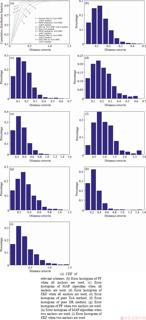
Figure 5 Distance error distributions of relevant schemes for Path 1:

Table 1 Mean error of all methods (m)

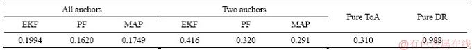
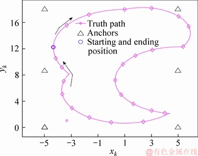
Figure 6 Path 2 setup for experiment

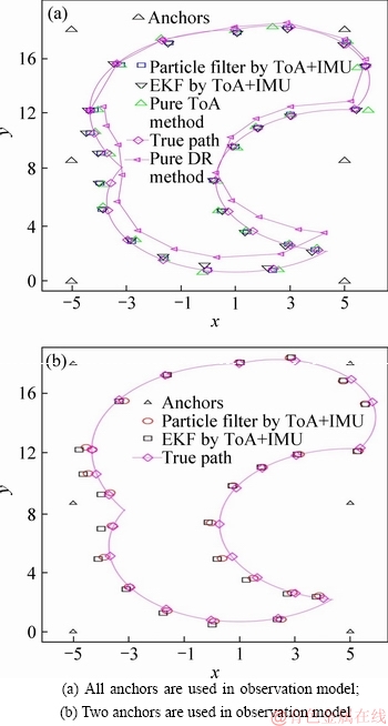
Figure 7 Comparisons between estimated paths and truth path for Path 2:

Table 2 summarizes the mean distance errors of various approaches in Path 2. Comparing Table 2 with Table 1 item by item, it can be seen that due to the characteristic of Path 2, pure DR method performs worse than the same method in Path 1 as more angle error is accumulated over the distance in Path 2. Thanks to the integration of WSN, the performance of hybrid methods does not deteriorate too much. When all anchors are used, both PF and EKF algorithms have less mean distance errors than the one of standalone ToA system. Reducing the number of anchors used to 2, the mean distance error of PF algorithm approximately equals the one of standalone ToA system.

Table 2 Mean error of all schemes (m)

5 Conclusions

Three different schemes on the basis of recursive Bayesian method are introduced. These three methods are capable to unitedly conduct inertial information and range measurements. All these methods do not require constant moving speed. In our simulation, it is obvious that the superiority of these schemes overs standalone ToA or standalone DR system. With them, EKF or PF methods can be applied for more general moving trajectories and still gain better performance than standalone schemes.

Figure 8 Distance error distributions of relevant schemes for Path 2:

Furthermore, researches are expected to apply the above systems to fit complex environments significantly, such as those scenarios where more barriers are included or electromagnetic interferences need to be considered.

References

[1] MAINETTI L, PATRONO L, SERGI I. A survey on indoor positioning systems [C]// IEEE International Conference on Software, Telecommunications and Computer Networks. Split, Croatia: Sep, 2014.

[2] LIU H, DARABI H, BANERJEE P, LIU J. Survey of wireless indoor positioning techniques and systems [J]. IEEE Transactions on Systems, Man, and Cybernetics: Part C (Applications and Reviews), 2017, 37(6): 1067-1080.

[3] MOSES R L, KRISHNAMURTHY D, PATTERSON R M. A self-localization method for wireless sensor networks [J]. EURASIP Journal on Advances in Signal Processing, 2003, 17(4): 839-843.

[4] KIM S, CHONG J W. An efficient TDoA-based localization algorithm without synchronization between base stations [J]. International Journal of Distributed Sensor Networks, 2015, 11(9): 832351. DOI: http://doi.org/10.1155/2015/832351.

[5] HUANG Y, ZHENG J, XIAO Y, PENG M. Robust localization algorithm based on the RSSI ranging scope [J]. International Journal of Distributed Sensor Networks, 2015, 11(2): 587318. DOI: http://doi.org/10.1155/2015/587318.

[6] ZHOU B, CHEN Q, XIAO P. The error propagation analysis of the received signal strength-based simultaneous localization and tracking in wireless sensor networks [J]. IEEE Transactions on Information Theory, 2017, 63(6): 3983-4007.

[7] NICULESCU D, NATH B. Ad hoc positioning system (APS) using AOA [C]// Twenty-Second Annual Joint Conference of the IEEE Computer and Communications. IEEE, 2003, 3: 1734-1743.

[8] SINGH M, BHOI S K, KHILAR P M. Geometric constraint-based range-free localization scheme for wireless sensor networks [J]. IEEE Sensors Journal, 2017, 17(16): 5350-5366.

[9] CHINTAKUNTA H, KRIM H. Divide and conquer: Localization coverage holes in sensor networks [C]// Proceedings of the 7th Annual IEEE Communications Society Conference on Sensor, Mesh and AdHoc Communications and Networks (SECON). Boston, USA, 2010: 1-8.

[10] COLLIN J, MEZENTSEV O, LACHAPELLE G. Indoor positioning system using accelerometry and high accuracy heading sensors [C]// Proc of ION GPS/GNSS 2003 Conference. 2003: 9-12.

[11] JIN Y, MOTANI M, SOH W S, ZHANG J. SparseTrack: Enhancing indoor pedestrian tracking with sparse infrastructure support [C]// INFOCOM, 2010 Proceedings IEEE. IEEE, 2010: 1-9.

[12] RUIZ A R J, GRANJA F S, HONORATO J C P, ROSASJ I G. Accurate pedestrian indoor navigation by tightly coupling foot-mounted IMU and RFID measurements [J]. IEEE Transactions on Instrumentation and measurement, 2012, 61(1): 178-189.

[13] LEE S, KIM B, KIM H, HA R, CHA H. Inertial sensor-based indoor pedestrian localization with minimum 802.15. 4a configuration [J]. IEEE Transactions on Industrial Informatics, 2011, 7(3): 455-466.

[14] WANG H, LENZ H, SZABO A, BAMBERGER J, HANEBECK U D. WLAN-based pedestrian tracking using particle filters and low-cost MEMS sensors [C]// Positioning, Navigation and Communications, 2007. WPNC'07. 4th Workshop on. IEEE, 2007: 1-7.

[15] RAI A, CHINTALAPUDI K K, PADMANABHAN V N, SEN R. Zee: Zero-effort crowdsourcing for indoor localization [C]// Proceedings of the 18th Annual International Conference on Mobile Computing and networking. ACM, 2012: 293-304.

[16] LATEGAHN J, MULLER M, ROHRIG C. Extended Kalman filter for a low cost TDoA/IMU pedestrian localization system [C]// Positioning, Navigation and Communication (WPNC), 2014 11th Workshop on. IEEE, 2014: 1-6.

[17] HU W Y, LU J L, JIANG S, SHU W, WU M Y. WiBEST: A hybrid personal indoor positioning system [C]// Wireless Communications and Networking Conference (WCNC), 2013 IEEE. IEEE, 2013: 2149-2154.

[18] CHEN X, SONG S, XING J. A ToA/IMU indoor positioning system by extended Kalman filter, particle filter and MAP algorithms [C]// Personal, Indoor, and Mobile Radio Communications (PIMRC), 2016 IEEE 27th Annual International Symposium on. IEEE, 2016: 1-7.

[19] MEMSIC Inc. DMU380ZA series user’s manual [M]. 2014.

[20] KALMAN R E. A new approach to linear filtering and prediction problems [J]. Journal of basic Engineering, 1960, 82(1): 35-45.

[21] JAZWINSKI A H. Stochastic processes and filtering theory [M]. Courier Corporation, 2007.

[22] ARULAMPALAM M S, MASKELL S, GORDON N, CLAPP T. A tutorial on particle filters for online nonlinear/ non-Gaussian Bayesian tracking [J]. IEEE Transactions on signal Processing, 2002, 50(2): 174-188.

(Edited by YANG Hua)

中文导读

混合无线传感网和惯性测量装置的室内定位系统

摘要：将惯性导航系统和无线传感网进行结合以提高室内定位的精度。惯性导航系统的关键装置为惯性测量装置，其用于测量附着的移动物体的加速度和旋转角。附着在移动目标上的传感器会通过时间到达法测量与事先放置的锚节点之间的距离。同时将加速度、旋转角和与锚节点之间的距离这些信息也被传到服务器终端以建立状态转移模型和观察模型，从而可以应用各种回归贝叶斯算法以实时估计出移动目标的位置。本文共提出应用三种回归贝叶斯算法。实验表明，这三种算法不仅不需要移动目标必须以匀速移动，而且均在定位精度方面优于单独的ToA定位方法和单独的步行者航位推算方法。而其中的两种方法可以用于以任何形式的轨迹曲线移动的目标定位，也就是不需要受到如下限制，两个连续的定位时间点之间通过的轨迹必须是直线。

关键词：室内定位；基于到达时间的测距法定位；贝叶斯滤波器；扩展卡尔曼滤波器；最大后验概率算法

Foundation item: Project(61301181) supported by the National Natural Science Foundation of China

Received date: 2018-09-07; Accepted date: 2019-06-20

Corresponding author: CHEN Xue-chen, PhD, Assistant Professor; Tel: +86-13824426548; E-mail: chenxch8@mail.sysu.edu.cn; ORCID: 0000-0002-7683-2933