
Modeling simulation and experimental validation for mold filling process
HOU Hua (侯 华) 1, JU Dong-ying(巨东英) 2, MAO Hong-kui(毛红奎) 1, D. SAITO 2
1. College of Materials Science and Technology, North University of China, Taiyuan 030051, China;
2. Department of Mechanical Engineering, Saitama Institute of Technology, Fusaiji, Saitama369-0239, Japan
Received 20 April 2006; accepted 30 June 2006
Abstract: Based on the continuum equation, momentum conservation and energy conservation equations, the numerical model of turbulent flow filling was introduced; the 3-D free surface vof method was improved. Whether or not the numerical simulation results are reasonable, it needs corresponding experimental validations. General experimental techniques for casting fluid flow process include: thermocouple tracking location method, hydraulic simulating method, heat-resistant glass window method and X-ray observation etc. The hydraulic analogue experiment with DPIV technique is arranged to validate the fluent flow program for low-pressure casting with 0.1×10⁵ Pa and 0.6×10⁵ Pa pressure visually. By comparing the flow head, liquid surface, flow velocity, it is found that the filling pressure value influences the flow state strongly. With the increase of the filling pressure, the fluid flow state becomes unstable, the flow head becomes higher, and the filling time is reduced. The simulated results are accordant with the observed results approximately, which can prove the reasonability of our numerical program for filling process further.
Key words: turbulent flow filling; VOF method; numerical simulation; experimental validation; DPIV
1 Introduction
Numerical modeling provides a powerful means of analyzing various complex phenomena, such as thermal flow, heat transfer and solidification as well as their coupling problems occurring during filling process of casting. Simulation allows researchers to observe and quantity what is not usually visible or measurable during real casting processes. The results of such simulations is to help shorten the design process and optimize conditions of casting process to reduce scrap, use less energy and, of course, make better filling process of casting[1]. Recently, numerical analysis method and modeling of the fluid flow for casting process has been studied in previous work[2-8]. Whether or not the numerical simulation results are reasonable, it needs corresponding experimental validations. General experimental techniques for casting fluid flow process include: thermocouple tracking location method, hydraulic simulating method, heat-resistant glass window method and X-ray observation etc .
In this paper, the hydraulic filling process is carried out to validate the thermal filling numerical simulation. In filling algorithm, the iterative times often extend to several thousands even millions, hence the computation efficiency is considerably low, so it is important to develop more efficient and precise arithmetic. In addition, casting filling experiments are usually difficult to carry out and simulation results are often unsatisfied etc.
2 SOLA method in numerical analysis of fluid
mechanics
Mass conservation and momentum conservation are represented by the continuum equation and N-S equation respectively as follows:
 (1)
(1)


 (2)
(2)
where U, V, W are the velocity components of x, y and z coordinates; ρ is the fluid density; p is the pressure; gx, gy and gz are the gravity accelerate velocities of x, y and z orientations; γ is the momentum viscosity. The weighting factor α is used to control the discrete format with α=0 representing the central difference format and α=1 representing the upper hand difference format. Here, Eqn.(1) is discrete by the central format and Eqn.( 2) is discrete by the upper hand format. The interleaving mesh is used to discrete the velocity and pressure for many advantages.
3 VOF method for free surface
There are many methods can deal with the free surface problem. The VOF(volume-of-fluid) method has been widely used for its short computational time. In VOF algorithm, the volume function should be solved, and then the filling state can be obtained, and so the new solution zone of velocity field and pressure field can be confirmed .
There is volume equation
 (3)
(3)
where F is the flow volume within one cell/volume of one cell, (0≤F≤1). When F=0, the cell is empty; when F =1, the cell is full of fluid; and when 0<F<1, there is some liquid in the cell, and the free surface exists.
The Donor-Acceptor method is adopted in VOF model to assure that the free boundary definition does not be damaged. Fluid flows out of the donor cells and into the acceptor cells. A plane passing through a cell, its orientation can be obtained by solving the normal vector representing the free surface in VOF method, and then we can determine the location of free surface according to F of the adjacent cells. For instance, when free surface is horizontal direction, compare F(i, j, k-1) and F(i j, k+1), if F(i, j, k+1)>F(i, j, k-1), consider that the fluid exists above the free surface, otherwise fluid exists below the free surface.
Since the “Donor-Acceptor” method is originally adopted in 1-D or 2-D simulations, in 3-D case, fluid can flow into or out of the six faces of a mesh unit simultaneously, so there will appear some “false” diffusions, and this method can bring some errors, even result in interface vague phenomenon. There have plenty of free surface units (0<F<1) between the full unit (F=1) and empty unit (F=0) along a certain direction, this kind of free surface units the more, the interface vague phenomenon is more serious.
With implicit method, in an arbitrary time step, there would be no empty units due to the false diffusion, which can result in serious interface vague. Otherwise, with explicit method, it is left empty since that the free surface carries only one unit forward in every time step, so interface vague do not be very serious. In order to get more actual free surfaces, author thinks that the explicit method must be adopted to describe the free surface of
0<F<1.
When fluid vontacts the wall during filling process, the thermal metal liquid would impact with the mould wall. This paper adopts a simple effective technique to treat this phenomenon .
The mould wall is acquiescently taken as a rigid wall in calculation as shown in Fig.1. When fluid flows to its right boundary or upper side boundary, there will be reflux. The diffusion of volume fraction function F follows such rule: firstly, F diffuses from (i+1, j) site to (i, j) site(here is the grid 1), if F of grid 1 is full or the returned F make the grid be full, and there is still surplus of F, then continue to diffuse to the below site, upper site and left site until return volume function had been distributed. The diffusion order of F is: 1-2-3-4 -5-6-7-8 to continue other domain number.
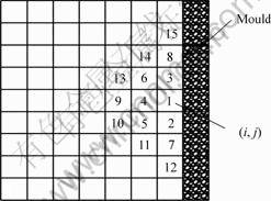
Fig.1 Collision between fluid and mould wall increase of calculation efficiency
Usually, it would take most time to solve the pressure and velocity field in filling process calculation. Some methods have been explored to improve the calculation efficiency with decreasing iteration frequency and quickening convergence speed. And now there are such methods as the conjugate gradient method, pre-treatment conjugate gradient method, dynamic relaxation factor method etc. Others also proposed mixture model to simplify the physical model and reduce calculation.
The internal and external area separation simplification algorithm is adopted in this paper.
The liquid metal filling area is divided into two parts: the internal unit and free surface unit. At every time step dt, free surface units move continuously forward, and form new free surfaces units to form new internal and external area as shown in Fig.2.
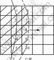
Fig.2 Chart of internal and external zone separation
With this scheme, the velocity, pressure contained in a unit doesn’t change again after the unit becomes an internal unit. All changes occur in the free surface units and their nearest units. The iteration calculation of speed and pressure is carried out in this area. As shown in Fig. 2, the iteration calculation at t+dt will be carried out only in the 1-10 units. So the grids number of participating in the iteration decreases greatly to raise calculation efficiency. Yet the absence of pressure and speed in the internal units can affect the calculation precision and flow state.
4 Principle of digital paraticle-image
velocimetry (DPIV)
Fig.3 presents the chart of the hydraulic analogue experiment with DPIV installation. This technology exploits the behavior of tracer particles added to a fluid flow, as the particles are very small and have nearly the same density as water, they act as flow followers in the local transient velocity field without disturbing the flow itself. Generally, a laser beam transformed into a thin plane of light illuminates a section of the flow containing a certain number of strongly reflective tracer particles. The illuminated particles are mapped on an image plane, and their positions are recorded by means of photographic plate, film, video, or a charge coupled device camera. From subsequent recordings with a known separation time ?t, a two-dimensional velocity pattern of the flow in the light sheet is determined.

Fig.3 Diagram of DPIV set
Owing to the successive illuminations, discrete images of the particles are recorded. At high seeding densities, however, “tracks” of individual particles cannot be identified, much less analyzed[9]. Hence, the mean displacement between successive illuminations of several particles in a so-called interrogation area has to be estimated. To this end, the image is digitized and the spatial correlation of the light distribution is calculated. With an interrogation area, the auto-covariance function is estimated by means of Fast Fourier Transforming (FFT) technology[10]. The mean displacement of the particles in the interrogation area between two successive illuminations is obtained from the shift in the peaks.
In this study, gas bubbles taken as particles are added to the water, a laser beam from 1.3 W argon-ion laser is transmitted onto the glass mold (as shown in Fig.3).
The size of the glass mould is 320 mm×280 mm×200 mm, its bottom ingate diameter is 30 mm. In calculation the mesh size is 5 mm×5 mm×5 mm, and the total meshes are 143 360. The water filling is carried out under 0.1×10⁵ Pa and 0.6×10⁵ Pa pressure. Here, the findings from the visualization experiments, from the simulation study, and from the DPIV measurements are mutually compared.
Fig.4 presents the observed (a1-h1) and simulated (a2-h2) surface waves under the pressure of 0.1×10⁵ Pa. Figs.2 (c3-g3) illustrate the observed streamlines. Figs.4 (a4-h4) show the simulated flow velocity evolution.
We can see from Figs.4(a1-h1) that, at beginning, the liquid surface is lower, and the flow head is bigger. With the increase of filling volume fraceion, the liquid surface ascends slowly and steadily, the flow head
become more and more plain and is submerged by surrounded water gradually, when the filling volume fraction arrives 50%, there is only a very small flow head, and the flow head disappears from the filling volume fraction 60% to the end.
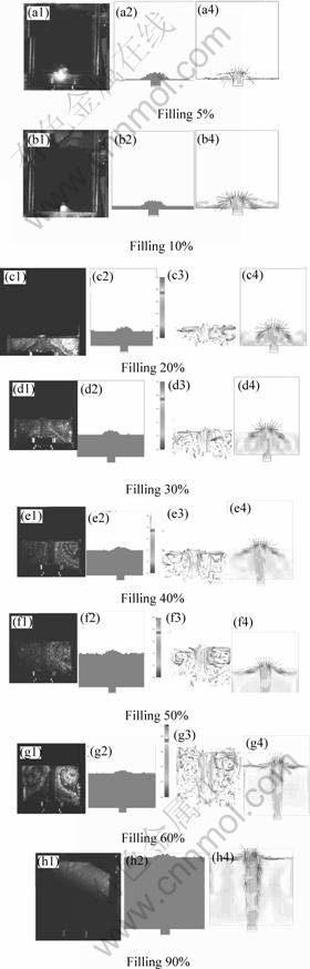
Fig.4 Comparison with observed and simulated filling process under pressure of 0.1×10⁵ Pa
In Figs.4(a2-h2), with the increase of filling volume fraction, the liquid surface ascends slowly and steadily, the flow head becomes more and more plain, which is approximately consistent with the observation from Figs.4(a1-h1), yet, the simulated flow head has not disappear until end.
In Figs.4(c3-g3), from the state of streamlines, we can see the flow state and the distribution characteristic of velocities. From Figs.4(c3-g3) and (c4-g4), we can see that, the simulated flow heads in Figs.(c4-g4) are more sticking out than that in Figs.(c3-g3), the simulated eddy currents at both sides of the core vertical upward stream are relatively weaker than that in Figs.(c3-g3). That is because in the experiment, there are two small metal columns at the bottom of the rectangle vessel, which can hinder the flow of the two sides’ liquid streams and cause the decomposition of the vertical upward speed to sides’ directions, so the flow head is lower and the eddy current is stronger. In calculation, the small cylinders are neglected for simplicity; so the simulated results are somewhat different with the experimental results.
In Figs.4(a4-h4), the direction and length of the arrow respectively represent the direction and magnitude of the velocity. It can be seen that the maximum velocity is in the center plane of the flow head and vertically upward. There have been velocity side components among the velocity of other positions. From the velocity vector distribution, it also can be found that, there exist some circuit flows around the flow head during the increase of the liquid surface. These are also accord with the DPIV results.
Although the simulated results and the DPIV findings do not agree completely in terms of the state of flow head, the trends are similar. Fig.5 presents the observed (a1-h1) and simulated (a2-h2) surface waves under 0.6×10⁵ Pa. Figs.3(a3-h3) show the simulated flow velocity evolution.
We can see from Figs.5(a1-h1) that, at beginning, the liquid surface is lower, and the flow head is quite bigger. With the increase of filling volume fraction, the liquid surface ascends with some little disturbance, the flow head is always sticking out obviously until the end.
The simulated results in Fig.5(a2-h2) are appro-ximately accordant with above experimental findings. It is different that the simulated liquid surface ascends quietly, yet, at present, there is no perfect mathematic model suitable for liquid surface vibration, and this numerical simulation study is still at the exploration stage, so the comparison of simulation and experiment is
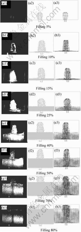
Fig.5 Comparison between simulated and observed filling process under 0.6×10⁵ Pa
main focused on the flow head and the eddy currents. Hence, the numerical method needs to be improved further.
In Figs.5(a3-h3), it can be seen that the maximum velocity is in the center plane of the flow head and vertically upward. There have been velocity side components among the velocity of other positions. From the velocity vector distribution, it also can be found that, there exist some circuit flows around the flow head during the increase of the liquid surface. These are also accordant with the DPIV results.
Although the simulated results and the DPIV findings do not agree completely in terms of the liquid surface, the trends are also similar.
Compared to the pressure of 1.0×10⁴ Pa, the differences of the center and surrounded velocities are obvious with that of 6.0×10⁴ Pa pressure.
Comparing Fig.4 with Fig.5, we can find that, the filling pressure value influences the flow state strongly. With the increase of the filling pressure, the fluid flow state becomes unstable, the flow head becomes higher, and the filling time is reduced.
Based on above discussions, it can be concluded that the simulated results are accordant with the observed results approximately, which can prove the reasonability of our numerical program.
References
[1] Hou H. Studies on Numerical Simulation for Liquid-metal Filling and Solidification During Casting Process[D]. Japan: Saitama Institute of Technology, 2005
[2] Hou H, Ju D Y, Zhao Y H, Cheng J. Numerical simulationfor dendrite growth of binary alloy with phase-field method[J]. J Mater Sci Technology, 2004, 20(12): 45-48.
[3] Hou H, Zhao Y H, Chu Z, Xu H. Numerical simulation of 3-D displacement fields of steel casting during solidification process[J]. Foundry Technology, 2002, (3): 145-149. (in Chinese)
[4] You B K. Temperature Measurement and Instrument: Couple and Thermal Resistance [M]. Document Press of Science and Technology, 1990.
[5] Compbell J. Invisible macrodefects on castings[J]. Journal de Physique iv, 1993(3): 861-872.
[6] Ju D Y , Inoue t. Simulation of solidification and heat flow in strip casting process by twin roll method[A]. Proceeding of Conference on Computer-assisted Design and Process Simulation[C]. Tokyo, 1993. 84-98.
[7] Ju D Y, Inoue t. Analysis of heat fluid flow incorporating solidification and its application to thin slab continuous casting process[J]. Transaction of the Japan Society of Mechanical Engineering (JSME), 1993, 59(565): 2189-2195.
[8] Kapranos P, Barkhudarov m r, Kirkwood d h. Modeling of structural breakdown during rapid compression of semi-solid alloy slugs[A]. 5th International Conference on Semi-solid Processing of Alloys and Composites[C]. Golden, 1998. 23-25.
[9] Hou HUA. Studies on Numerical Simulation for Liquid-metal Filling and Solidification During Casting Process[D]. Japan: Saitama Institute of Technology, 2005.
[10] Wester j. Delft University of Technology[D]. Delft, Netherlands: Delft University of Technology, 1993.
(Edited by CHEN Ai-hua)
Corresponding author: HOU Hua; Tel: +86-13934153099; E-mail: houhua@263.net

