Indoor moving vehicle detection by trajectory matching

CHEN Yi-hong(陈毅鸿)¹, Felix Lütteke², CHEN Qi-jun(陈启军)¹, J?rg Franke²

(1. School of Electronics and Information, Tongji University, Shanghai 201804, China;

2.The Institute of Manufacturing Automation and Production Systems,

Friedrich-Alexander-Universit?t Erlangen-Nürnberg, Erlangen 91058, Germany)

Abstract: A solution to determine the positions of transportation vehicles without any optical markers in an area under camera surveillance was introduced. This solution was based on a net of cameras on the ceiling of the vehicle operational areas. A robust background subtraction method was performed to detect the contours of all moving objects in every camera frame. These so called foreground objects contours were fed into a particle filter to estimate the position, orientation and speed of the detected objects over a certain number of frames. Based on the camera data this so-called state estimation was performed for all foreground objects like humans, other moving obstacles and the vehicles. Due to the fact that the vehicles can be totally covered by their payload, they cannot be detected by color or shape. Instead, the vehicles were identified by comparing their movement with the movement of all detected foreground objects.

Key words: background subtraction; hungarian algorithm; particle filter; trajectory matching; similarity

CLC number:TP24             Document code: A            Article ID: 1672-7207(2011)S1-0561-06

1 Introduction

To perform automated material transport in production plants, automated guided vehicles (AGV) are often deployed. Depending on the technical level, these vehicles can be guided by fixed guidelines. Technical realizations are optical guidelines or inductive guidelines. More sophisticated systems are predicated on autonomous vehicles that do not need any fixed guidelines. Instead, these highly flexible transportation vehicles are capable of performing a transportation task automatically. Prerequisites for this are the mechanisms to detect the position and map of the environment of the vehicles. To fulfill these requirements, modern autonomous vehicles rely on complex local sensors like laser scanners for obstacle detection and self localization. This increases the cost for each vehicle, keeping low infrastructural costs.

Another approach to autonomous transportation is to install a global camera. Thereby vehicle costs can be significantly reduced, although infrastructural invest raises. That’s why this concept is advantageous if many small scale vehicles are operating in a small area. In this work a mechanism was suggested to localize and track the vehicles even if they have no optical markers and no predefined shape. The hardware setup of the system is shown in Fig.1. The camera images were sent to a computer so-called world model server to calculate a mathematical representation of the environment of the vehicle. In addition the vehicle sent its local sensor data to the world model server. This information was merged in the world model server to obtain a precise mathematical representation of the so-called world model. It provides information about all detected objects robust background substraction^[1] and distinguishes obstacles from the vehicle itself by particle filter^[2]. Finally the world model was transmitted to the vehicle, enabling it to carry out its transportation tasks autonomously.

Nowadays, object detection is used widely in many fields like face detection and ball detection in robot’s soccer competitions^[3]. Generally speaking, vision tracking of objects can either be based on the detection of some markers^[3] or scale-invariant feature transform (SIFT)^[4]. In this case special geometric features of the objects are tracked. Both algorithms have the necessary condition that the tracked object is directly visible by the camera. As the transportation vehicles can be covered by their payload, situations can occur when neither the vehicles’ color nor their shape can be detected. With the proposed vehicle detection system the vehicles can be tracked anyway. This is done by matching the trajectory of the vehicles to the best fitting trajectory of the detected objects. Figure 2 shows how a set of images of the real world and the locally recorded trajectory of the vehicles are processed to yield a state-estimation of all dynamic obstacles and the vehicles in the monitored area. This algorithm can be divided into four parts: 1) Find all contours including position and size from the current frame of the global cameras; 2) Assign the found contours to predicted positions of the objects of the world model; 3) Use the assigned contours to enhance the state estimation of all objects by feeding the data into a particle filter; 4) Find the vehicles among the detected objects by comparing the trajectory of all objects with the trajectories of all vehicles. In Section 2, these four parts will be introduced in detail.

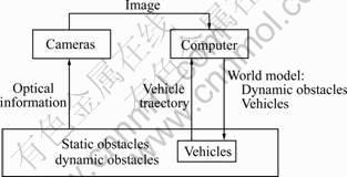
Fig.1 Hardware setup of proposed vehicle tracking system

Fig.2 Data processing in proposed vehicle tracking system

2 Algorithm

2.1 Image processing

The image processing step is aimed on image segmentation^[5], means to divide the image into different regions^[6]. In the current computer vision algorithms the similarity of image parts is usually defined in terms of color and texture. The proposed vehicle system is aimed on indoor operation with constant environmental conditions. Because of this, background subtraction methods can result in good object detection. In the test system, static objects will be included in the background thereby removing them from the global map. The handling of static objects is not in the focus of this work. For simplicity, it is assumed that no static obstacles exist in the operational area of the vehicles. The basic idea of background subtraction is to detect the foreground objects as the difference between the current frame and an estimation of the scenes static background. Equation shows the way to generate a binary image by background subtraction of a gray image with pixels g_f and a gray image background estimation with pixels g_b. Depending on the threshold value g_t, each pixel is either regarded as background or foreground.

2.2 Assign contours to existing objects

After processing the image to obtain all contours, these contours have to be assigned to the existing objects. The particle filter provides a prediction for each objects state. This prediction consists of the position  for time step k. The found contours in the frame F(k), in the following called measurement, will be used to improve the current position estimation of the objects. Figure 3 illustrates the special case that the number of the found contours correspond to the number of predicted object positions. It can be seen that the values of the position prediction p_i shown in Fig.3(a) are different from the position measurement depicted in Fig.3(b). These distances are written to the nonnegative matrix C₀:

C₀=(c_ij)                 (2)

where c_ij describes the distance between prediction p_i and measurement m_j. Due to noise and other disturbances in the image recording process, the number of measurements n_m is different from the number of predictions n_p. In this case, C₀ is not a square matrix. To be able to apply well known algorithms to find an optimal assignment, C has to be square. Depending on the number of predictions n_p and measurements n_m, zeros are added to C₀ to yield a square matrix C:

(1) n_p≤n_m: By concatenating a (n_m-n_p)×n_m zero matrix to C₀ (n=n_m), a n×n matrix C is obtained:

                (3)

The distance matrix C₀ is enhanced by n_m-n_p fictive position predictions. The fictive distance of these predictions to all position measurements is set to 0. These fictive predictions will be assigned to the position measurements that fit the least to the existing position predictions.

Fig.3 Position prediction and measurement for n_p=n_m=2

 (2) n_p>n_m: By concatenating a n_m×(n_p-n_m) zero matrix to C₀ (n=n_p), a n×n matrix C is obtained:

               (4)

A binary matrix X=(x_ij) is introduced

   (5)

The aim is to find the matrix X that minimizes the following expression:

               (6)

with the additional constraints:

       (7)

         (8)

         (9)

Equation (9) makes sure that only one prediction is assigned to each measurement and vice versa. The minimization of Eq.(6) describes a typical minimum cost flow problem which in turn is a special case of a linear assignment problem (LAP)^[7]. The Hungarian algorithm^[8] is one of the algorithms that have been devised to solve the linear assignment problem. However, the result is a binary matrix X that assigns every prediction to a single measurement.

As shown in Fig.4, the assignment can even comprise fictive predictions and measurements. If the number of measurements exceeds the number of predictions as shown in Fig.5, fictive predictions are assigned to n_m-n_p measurements. These measurements can be treated as new detected objects. If the number of predictions exceeds the number of measurements as shown in Fig.6, fictive measurements are assigned to n_p-n_m predictions. These predictions can be treated as disappeared objects. Because this work does not focus on the handling of new objects and deletion of existing objects, this process is not explained in detail here.

2.3 Particle filter

In order to obtain a smooth position estimation of the objects and to estimate the speed and orientation which in turn are necessary to compute a good prediction of the next object position, a state estimator is implemented. A popular technique for state estimation is the particle filter^[2]. It represents the state estimation by a number of points in the given state space. These points are called particles. The accuracy and computational load can be easily adjusted by changing the number of particles for the filter. Figure 7 shows the steps of the basic algorithm.

Fig.4 Result of assignment process for two position predictions and position measurements

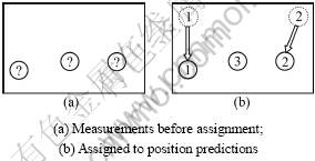
Fig.5 Assignment of position measurements to predictions with n_pm

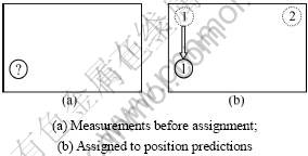
Fig.6 Assignment of position measurements to position predictions with n_p>n_m

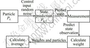
Fig.7 Schematic diagram of particle process

The basic algorithm consists of the following steps: (1) All particles are changed due to the current state (like velocity, acceleration and so on) and current control input u. In addition some random noise is added to the states to modify each particle individually; (2) Compare the resulting state estimations with the measured position; (3) Assign weights to the particles depending on the difference between measurement and prediction; (4) Draw n particles with replacement from the existing population P to gain a new population P+. The probability for a particle to be drawn is proportional to its weight; (5) From the existing particle distribution, calculate a reasonable state estimation (e.g. average over all particles, choose the area with the highest density of particles). To be able to perform step 1, a mathematical model of the system comprising the desired states needs to be set up. The state vector of the vehicle is shown in Eq.(10).

           (10)

where x, y and θ describe the current position and orientation of the vehicle. In addition, the longitudinal velocity v, and the time derivative of the orientation  are estimated.

Figure 8 gives the relation between these physical values. The position and orientation at time t are described by the following equations:

        (11)

      (12)

           (13)

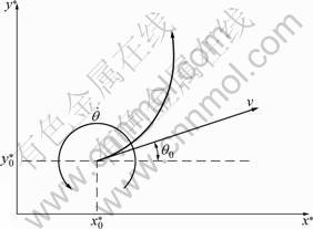
Fig.8 Model of vehicle motion used in proposed particle filter

Position and orientation are calculated based on the assumption that both velocity v and change in orientation    do not change with time. This assumption is in general not correct but enables us to calculate a state prediction for the future. Solving the integrals in Eqs.(11)-(13), replacing t with Δt and x₀, y₀ and  with x_k, y_k and   yields a time discrete description of the desired model:

    (14)

   (15)

            (16)

               (17)

               (18)

Equations (14)-(18) describe the prediction of the state vector depending on the state at time step k. Equations (17) and (18) describe the assumption that v and  do not change with time. By implementing this model with a standard particle filter the following results can be observed: (1) Particles will move towards real state in state space, and velocity v and change of orientation  will be estimated in a good way even though they are not measured; (2) As the model is based on the assumption that v and  are constant, the best estimation result is obtained when the vehicle drives in a circle, thereby fulfilling the proposed assumptions.

2.4 Match

The above sections describe an algorithm to obtain a stable estimation of all object positions in the operational area of the vehicles. Finally a method is introduced, that assigns the vehicles to their representation as objects in the world model server. To do so, the trajectory of each vehicle is compared with the trajectories of all objects. The object with the most similar trajectory to the one of the regarded vehicle is assumed to represent the vehicle itself. Figure 9 shows the relative position of the vehicles in local coordinate system x′ and y′ in the global coordinate system x^* and y^* depending on , and θ₀. During trajectory matching the relative positions of both coordinate systems are constant. All waypoints in the local coordinate system can be projected into the global coordinate system with the following equation:

   (19)

where θ₀ is the rotation of the local coordinate system and p₀ is the proportional factor that describes the sizing between two trajectories. It is now intended to find the four parameters x₀, y₀, θ₀ and p₀.

             (20)

              (21)

Fig.9 Relative position of vehicles local coordinate system x′, y′ and global coordinate system x^*, y^*

Equation (19) can be written in a simplified form:

(22)

By extending the scalars x^*, y^*, x′, y′ to q×1 vectors X^*, Y^*, X′ and Y′ containing q points of the global and the local trajectory respectively and replacing 0 with a column vector Z of q zeros as well as replacing 1 by a column vector O consisting of q ones, in case of q>2, an over determined equation system is obtained:

       (23)

To yield a result for a₀, b₀, x₀ and y₀, Eq.(23) can be solved in terms of minimum square error. This can be achieved by applying the pseudo inverse to Eq.(24) to solve a₀, b₀, x₀ and y₀.

The values for a₀, b₀, x₀ and y₀ describe the optimal transformation of the trajectories from one coordinate system to another according to Eqs.(23) and (24).

    (24)

If the rotation of the local coordinate system θ₀, as well as the proportional factor p₀ are needed, solving Eqs.(20) and (21) gives the desired result:

              (25)

            (26)

Finally the error value needs to be calculated to gain a value for the similarity of the compared trajectories. Therefore the projection [X_p Y_p] of the trajectory in the local coordinate system into the global coordinate system according to Eq.(23) is calculated. The squared distance between all points of the trajectory in the global coordinate system and the projected points is summed up and divided by the number of points q.

            (27)

The smaller this error is, the more likely the compared trajectories of object and vehicle belong to each other.

3 Experiment

To demonstrate the presented algorithm, a small scale prototype transportation vehicle was set up. The camera is a standard webcam with a resolution of 320×240 pixels. It is set to a fixed sample rate of 1 frame per second Δt=1 s. The number of waypoints q per trajectory is set to 15. So the vehicle will run in a circle with constant speed for 15 s and stop afterwards. For testing reasons two objects trajectories are sampled during these 15 s. Figure 10 shows the basic setup. Static obstacles are surrounded by white rectangles and belong to the background. They will not appear as object in the image process. The obstacle is surrounded by a black rectangle belonging to the foreground. Its representation as object 2 in the world model server will not move significantly. Its movement results from the noise in the camera images and particle filter. The vehicle also belongs to the foreground. It will be represented as object 1 in the world model server. Figure 10(b) shows the vehicle on its way, driving a circle. In Fig.10(c), the vehicle has completed its path. Now the recorded trajectories of the not moving object and the moving object can be compared with the trajectory, and the vehicle recorded with its onboard incremental encoders. Eq.(27) is used to find the vehicle, Fig.10(c) shows that the vehicle is detected and located, and Figs.11 and 12 show the calculations. In Fig.11 the result of the comparison of the trajectory of object 1 with the vehicle trajectories is shown. The optimal projection of the vehicle trajectories into the global coordinate system is shown as solid line. The dotted line is the trajectory of the moving object. It can be observed that the estimated object trajectory is not a perfect circle. This is resulted from the noise in the camera images and the particle filtering, as particles in the state space first have to converge to the correct state comprising speed v and rotational speed  Still the result according to Eq.(27) is quite a small error of e=0.201 9 m². Fig.12 depicts the results of the comparison of the vehicle trajectories with the trajectory of object 2. Again the solid line is the optimal projection of the vehicles trajectory into the global coordinate system while the dotted line shows the movement of the object. Here, the result from Eq.(27) indicates an error of e=1.65 m². According to these results it seems very likely, that object 1 is the representation of the vehicle. This hypothesis can be further confirmed by tracking the trajectories of vehicle and assigned object.

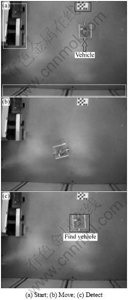
Fig.10 Experimental validation of proposed vehicle tracking algorithm

Fig.11 Comparison of projected vehicle sensor data with recorded trajectory of object 1

Fig.12 Comparison of projected vehicle sensor data with recorded trajectory of object 2

4 Conclusions

The theoretically devised method to track objects with cameras without any knowledge of their color or shape is tested in an artificial testing environment. A moving object can be assigned to a given trajectory. Further work needs to be done in the image processing to get a more stable estimation of the background if environmental conditions change. This would lead to a more precise object position estimation and thereby could lead to smaller errors in the assignment of the trajectories.

References

[1] Stauffer C, Grimson W. Learning patterns of activity using real-time tracking [J]. IEEE Transactions on Pattern Analysis and Machine Intelligence, 2000,22(8): 747-757.

[2] Thrun S, Burgard W, Fox D. Probabilistic Robotics[M]. Cambridge: The MIT Press, 2005: 237-279.

[3] R?fer T, Laue T, Müller J, et al. B-human team report and code release 2010[EB/OL]. http://www.b-human.de/filedownload/33/ bhuman10coderelease.pdf.

[4] Lowe D. Object recognition from local scale-invariant features [J]. IEEE Computer Society, 1999: 1150.

[5] Gonzalez R, Woods R, Eddins S. Digital image processing using MATLAB[M]. New Jersey: Prentice Hall Upper Saddle River, 2004: 624.

[6] Fu K, Mui J. A survey on image segmentation[J]. Pattern Recognition, 1981, 13(1): 3-16.

[7] Jonker R, Volgenant A. A shortest augmenting path algorithm for dense and sparse linear assignment problems[J]. Computing, 1987, 38(4): 325-340.

[8] Kuhn H. The Hungarian method for the assignment problem[J]. Naval Research Logistics Quarterly, 1955, 2(1/2): 83-97.

(Edited by HE Yun-bin)

Received date: 2011-04-15; Accepted date: 2011-06-15

Foundation item: Projects(2010DFA12210, 2009DFA12520, 10160704500) supported by International Cooperation; Project(2009AA043001) supported by the National High Technology Research and Development Program of China; Project(10511501002) supported by Shanghai Science and Education Reserch Program

Corresponding author: CHEN Qi-jun, Professor, PhD; Tel: +86-21-69589338; E-mail: qjchen@tongji.edu.cn