Unknown input reconstruction based on auxiliary output

HAN Dong(韩冬), ZHU Fang-lai(朱芳来), YANG Jun-qi(杨俊起)

(College of Electronics and Information Engineering, Tongji University, Shanghai 200092, China)

Abstract: A lot of methods were proposed to design observer for reconstructing the unknown input when the so-called observer matching condition was met. The problem of designing observer and reconstructing the unknown input was considered when the system does not meet the condition. The idea of generating auxiliary outputs was adopted to meet the matching condition. Then the high-gain observer was used to obtain the estimates of auxiliary outputs by which a reduced-order observer is designed to estimate the unknown input. The simulation results of a real model show that the proposed method is effective.

Key words: unknown input reconstruction;observer matching condition; reduced-order observer; high gain observer

CLC number: TP391             Document code: A            Article ID: 1672-7207(2011)S1-0633-05

1 Introduction

To estimate the unknown input is one of the most important problems in modern control theory. For example, the cutting force exerted by the machine tool is difficult or sometimes very expensive to measure. If we regard the cutting force as an unknown input to the machine tool system, it is quite meaningful to construct an observer which can estimate it.

The early work of unknown input observer (UIO) design can be traced back to the seventies of the last century^[1-2]. The literatures^[3-5] present some direct design procedures of full-order and reduced-order observers for linear systems with unknown inputs. In Ref.[16], the concept of the input observability is given and a systematic and simple approach to the design of schemes for input reconstruction is developed. HA et al^[17] discusses the problem of estimating simultaneously the state and input of a class of Lipschitz nonlinear systems and the observer design problem can be solved via a Riccati inequality or a LMI based technique.

The necessary and sufficient conditions to construct an unknown-input observer is that the invariant zeros of the system must lie in the open left half complex plane, and the observer matching condition is satisfied^[4]. The work mentioned above were all accomplished under the circumstances that the system meets the two conditions. But for many dynamic systems the second condition is too harsh.

In this work, the idea of generating auxiliary outputs from Ref.[8] was adopted. High-gain observers^[9] are then used to obtain the estimates of these auxiliary outputs which can be used in a reduced-order observer designing^[4] and in estimating the unknown input ^[3].

2 Reduced-order observer design and unknown input reconstruction

2.1 Background statements

Consider the linear time-invariant system

       (1)

where ,,, are the state vector, output vector, known input vector, unknown input vector, respectively. , ,  and  are constant matrices. Without loss of generality, assume ,,.

Assumption 1 The system (1) is minimum phase, i.e. the invariant zeros of the triple all in the open left-hand complex plane，or for all complex number s，when, the following Eq.(2) holds.

     (2)

Assumption 2 .

Assumption 3 , i.e. the unknown input is bounded.

Remark1 Assumption 1 is a necessary condition for designing the observer.

when, we say that the system (1) meets the so-called observer matching condition. Many methods ^{[2-4, 10-14]} were proposed to design the observer with unknown input when Assumption 1 and the observer matching condition are met. The main purpose of this paper is to design an observer to estimate the unknown input by constructing auxiliary output when even the system does not meet the so-called observer matching condition.

2.2 Estimation of auxiliary output

Floquet et al^[8] proposed a method to design auxiliary output based on the concept of relative degree. The relative degree of the i-th output y_i with respect to the unknown input u₂ is defined to be the smallest positive integer r_i which makes the follwing eqhation hold:

 ,

where c_i is the i-th row vector of C.

There exists () such that the following auxiliary output matrix               , where

,

meets the observer matching condition, that is,

.

Now we consider the system with auxiliary output

         (2)

The invariant zeros of the triples  and are identical [8].

Differentiate  () with respect to time t, we have

If we denote

, , ,

Then we have , where . If ,  is the -th output of original system and it is , of course, measurable. For those , the   dynamics  of   are  given  by

          (3)

where .

For Eq. (3), we can construct the following high-gain observer

       (4)

where  and  is Hurwitz.

From Eqs. (3) and (4) we get

            (5)

where , .

Let with , , we get  and then  such that , where

It follows from Eq. (5) that we have

Where

The above equation can be rewritten as

       (6)

Obviously, all the eigenvalues of M_i are in the left-hand complex plane. From assumption 3, we know that the second item of right side of Eq. (6) is bounded.

Theorem 1^[15]:  For the high-gain observer (4), there exist a positive constant  and a finite time  such that  for . Moreover, .

From theorem 1, it is obviously that when  such that , then ，.

It follows from  that

                (7)

where

, , .

Note that . Let  and  if . It follows from Lemma1 that after a finite time , such that

               (8)

where

, moreover, .

In order to eliminate the peaking phenomenon of the high-gain observer [13], it is necessary to saturate the estimate . If , we have

with , . If , then . Thus, we get the saturation of  , that is, .

3 Reduced-order observer design

3.1 Reduced-order observer design

For newly constructed system (2), as , so we can construct a nonsingular matrix  with , then Eq. (2) can be transformed into:

            (9)

with , , where

, ,

,,

We then get an unknown-input-free sub-system as

    (10)

Since matrix  has full column rank, then there exists a nonsingular matrix with , We denote  with  and , so, we get

And pre-multiplying both sides of measurement Eq. (10), we get

           (11)

And by substituting, we get

       (12)

where

, ,

, .

Theorem 2: For system (2), if  is measurable and the pair  is observable or detectable, the following observer can asymptotically estimate the states of Eq. (2) with ,.

 (13)

Proof The pair  is detectable or observable^[3], following the conventional Luenberger design procedure, we can design observer for Eq. (12) as

By selecting  properly such that all the eigenvalues of  can be placed in the open left-hand complex plane.

Then  for . Following Eq. (13), we get . Since , so .

Now, we employ  instead of  to design the reduced-order observer

3.2 unknown input reconstruction

We reconstruct the unknown input based on the reduced-order observer with auxiliary output which is designed above.

    (14)

where

It is notice that the derivative information of the auxiliary output vector appears in Eq. (14) and solve numerical derivative problems for function with the first-order three points derivative formula for at points t_i () as following

Now we can give the numerical solution algorithm:

Step 1 Dividing the time interval  into N parts which is equivalent each other produces N+1 times points of  ();

Step 2 Setting the initial states of  and using Runge-Kutta method [16] give (). Discrediting  at time  yields . By the second equation of (11), we compute out .

Step 3 By Eq. (13), we compute out ;

Step 4 Setting () to yields the numerical solution of

4 Simulation and analysis

Consider the following linear, time-invariant system

,,

Obviously, . Thus, we choose  such that

,

are full ranks with . A high-gain observer was employed to estimate the auxiliary output. Let ,, then give the reduced-observer design as following:

And, the unknown input reconstruction is as follows:

The approximation of can be calculated with the numerical solution algorithm discussed above.

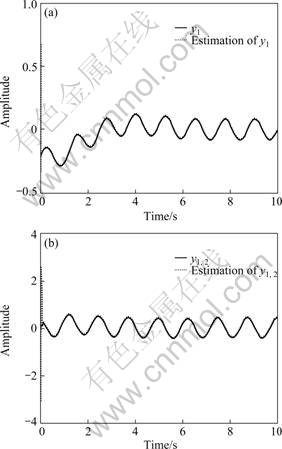
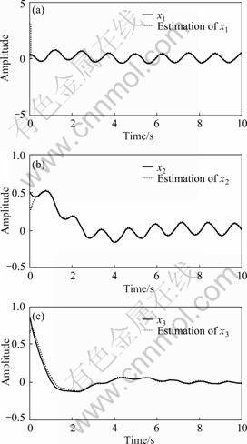
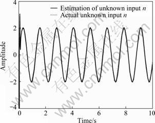
The auxiliary output estimation, state estimation and unknown input reconstruction are shown in Figs. 1-3. It can be found that the simulation results are satisfactory.

Fig.1 Curves of auxiliary output y_a and its estimation

Fig.2 Curves of state x and its estimation

Fig.3 Curves of unknown input u₂ and its reconstruction

5 Conclusions

The idea of generating auxiliary outputs were adopted when the system cannot meet the observer matching condition. Then the high-gain observers were used to obtain the estimates of these auxiliary outputs which can be used in a reduced-order observer designing and in estimating the unknown input. The simulation results to a real model show that the proposed method is effective.

References

[1] Wang S H, Davison E J, Dorato P. Observing the states of systems with unmeasurable disturbances[J]. Trans Automat Contr.

[2] Bhattacharyya P. Observer design for linear systems with unknown inputs[J]. Trans Automat Contr, 1978, AC-23: 483-484.

[3] Hou M, Muller P C. Design of observers for linear systems with unknown inputs [J]. IEEE Transactions on Automatic Control, 1992, 37(6): 871-875.

[4] Darouach M , Zasadzinski M[J]. Xu S J. Full-order observer for linear systems with unknown inputs. IEEE Transactions on Automatic Control, 1994, 39(3): 606-609.

[5] Yang F, Wilde R W. Observer for linear systems with unknown inputs[J]. IEEE Transactions on Automatic Control, 1988, 33(7): 677-681.

[6] Hou M, Patton R J. Input observability and input reconstruction[J]. Automatica, 1998, 34(6): 789-794.

[7] Ha Q P, Trinh H. State and input simultaneous estimation for a class of nonlinear systems[J]. Automatica, 2004, 40: 1779-1785.

[8] Floquet T, Edwards C, Spurgeon S K. On sliding mode observers for systems with unknown inputs[J]. International Journal of Adaptive Control and Signal Processing, 2007, 21: 638-656.

[9] Mahmoud N A, Khalil H K. Asymptotic regulation of minimum phase nonlinear systems using output feedback[J]. IEEE Transactions on Automatic Control, 1996, 41(10): 1402-1412.

[10] Kudva P, Viswanadham N, Ramakrishna A. Observers for linear systems with unknown inputs[J]. IEEE Trans Automat Contr, vol. ACS.

[11] Miller R J, Mukundan R. On designing reduced-order observers for linear time-invariant systems subject to unknown inputs[J]. Int J Contr, 1982, 35: 183-188.

[12] Kobayashi N, Nakamizo T. An observer design for linear systems with unknown inputs[J]. Int J Contr, 1982, 1982, 35: 605-619.

[13] Fairman F W, Mahil S S, Luk L. Disturbance decoupled observer design via singular value decomposition[J]. ZEEE Trans Automat Contr, 1984, AC-29: 84-86.

[14] Hostetter G, Meditch J S. Observing systems with unmeasurable inputs[J]. IEEE Trans Automat Contr, 1973, AC-18: 307-308.

[15] Kalsi K, Lian J, Hui S, et al. sliding-mode observers for systems with unknown inputs[EB/OL]. http://cobweb.ecn.purdue.edu/ ~zak/UIO_SMO_TAC.pdf, 2008.

[16] Zhang W, Li T. Numerical analysis[M]. Beijing: Beijing University Press, 2007.

(Edited by LONG Huai-zhong)

Received date: 2011-04-15; Accepted date: 2011-06-15

Foundation item: Project (61074009, 60972035) supported by the National Nature Science Foundation of China; Project (B004) supported by Shanghai Leading Academic Discipline Project

Corresponding author: HAN Dong; Tel: 15201962477; E-mail: handong2007@163.com