J. Cent. South Univ. (2020) 27: 780-796

DOI: https://doi.org/10.1007/s11771-020-4331-0

Pressure transient analysis of a finite-conductivity multiple fractured horizontal well in linear composite gas reservoirs

REN Jun-jie(任俊杰)^{1, 2}, GAO Yang-yang(高洋洋)¹, ZHENG Qiao(郑桥)¹,GUO Ping(郭平)³, WANG De-long(王德龙)⁴

1. School of Sciences, Southwest Petroleum University, Chengdu 610500, China;

2. Institute for Artificial Intelligence, Southwest Petroleum University, Chengdu 610500, China;

3. State Key Laboratory of Oil and Gas Reservoir Geology and Exploitation, Southwest Petroleum University, Chengdu 610500, China;

4. Research Institute of Exploration & Development of Changqing Oilfield Company, PetroChina,Xi’an 710018, China

Central South University Press and Springer-Verlag GmbH Germany, part of Springer Nature 2020

Abstract: Faulted gas reservoirs are very common in reality, where some linear leaky faults divide the gas reservoir into several reservoir regions with distinct physical properties. This kind of gas reservoirs is also known as linear composite (LC) gas reservoirs. Although some analytical/semi-analytical models have been proposed to investigate pressure behaviors of producing wells in LC reservoirs based on the linear composite ideas, almost all of them focus on vertical wells and studies on multiple fractured horizontal wells are rare. After the pressure wave arrives at the leaky fault, pressure behaviors of multiple fractured horizontal wells will be affected by the leaky faults. Understanding the effect of leaky faults on pressure behaviors of multiple fractured horizontal wells is critical to the development design. Therefore, a semi-analytical model of finite-conductivity multiple fractured horizontal (FCMFH) wells in LC gas reservoirs is established based on Laplace-space superposition principle and fracture discrete method. The proposed model is validated against commercial numerical simulator. Type curves are obtained to study pressure characteristics and identify flow regimes. The effects of some parameters on type curves are discussed. The proposed model will have a profound effect on developing analytical/semi-analytical models for other complex well types in LC gas reservoirs.

Key words: semi-analytical model; linear composite gas reservoir; multiple fractured horizontal well; finite-conductivity hydraulic fracture; pressure behavior

Cite this article as: REN Jun-jie, GAO Yang-yang, ZHENG Qiao, GUO Ping, WANG De-long. Pressure transient analysis of a finite-conductivity multiple fractured horizontal well in linear composite gas reservoirs [J]. Journal of Central South University, 2020, 27(3): 780-796. DOI: https://doi.org/10.1007/s11771-020-4331-0.

1 Introduction

Faults are very common in various gas reservoirs, and some leaky faults have an important influence on the development of faulted gas reservoirs. Owing to the existence of leaky faults, the gas reservoirs are usually divided into several reservoir regions with different properties, and the gas in one reservoir region can flow cross the faults and go into other reservoir regions. Therefore, the influence of leaky faults on fluid flow has attracted much attention. Linear composite (LC) model is considered as a reasonable approximation for describing fluid flow in hydrocarbon-bearing reservoirs separated by linear faults [1, 2]. In the last few decades, composite models, mainly including radial composite (RC) models and linear composite (LC) models, have been widely investigated and applied to various oil and gas reservoirs with variable reservoir properties. However, most of studies focus on RC models [3-5] and studies on LC models are few.

Pressure transient analysis is considered as a good way to analyze fluid flow characteristics and reservoir/well properties [6-15]. Pressure response of vertical wells in LC reservoirs has been investigated since the early 1960s. BIXEL et al [16] proposed the first analytical model of vertical wells in LC reservoirs and studied the impact of the fault on pressure behaviors. YAXLEY [1] developed an analytical model for LC reservoirs with a partially communicating fault. AMBASTHA et al [17] extended the LC model for infinite reservoirs to the one for finite strip reservoirs. BOURGEOIS et al [18] developed an analytical model for 3-zone LC reservoirs. KUCHUK et al [19] further developed an analytical model for n-zone LC reservoirs. ANDERSON [20] proposed an explicit analytical solution for fluid flow in infinite aquifers with a fault, and investigated the effect of the anisotropic fault. EZULIKE et al [21] developed an analytical model of horizontal wells in LC reservoirs, and investigated pressure behaviors of horizontal wells. ZEIDOUNI [22, 23] proposed analytical and semi-analytical models of vertical wells in multilayer reservoirs with a leaky fault, respectively. FENG et al [24] developed an analytical model of a vertical well in a dual-porosity LC reservoir, and studied the characteristic of pressure behaviors. Considering fault permeability alteration, MOLINA et al [2] proposed an analytical model of vertical wells in LC reservoirs and used it to detect the fault reactivation. However, until now, almost all of analytical/semi-analytical models for LC reservoirs were aimed at vertical wells, and the studies on complex well types in LC reservoirs are rare. Compared with the establishment of analytical/ semi-analytical RC models for complex well types, it is much more difficult to establish analytical/ semi-analytical LC models for complex well types. Therefore, there are still significant challenges in establishing analytical/semi-analytical models for complex well types in LC reservoirs, for example, multiple fractured horizontal (MFH) wells with finite-conductivity hydraulic fractures.

Horizontal well in combination with hydraulic fracturing is considered as a good means of developing various oil/gas reservoirs, especially low-permeability oil/gas reservoirs. In the last decade, tight oil/gas reservoirs have captured the attention of people owing to the enormous oil/gas reserves, and MFH well has been extensively employed to develop these ultra-low-permeability reservoirs. Of course, the MFH well is not merely applied to low-permeability reservoirs; it is also used to develop some mid/high-permeability reservoirs because it can significantly increase production at low cost. Therefore, a variety of analytical/semi-analytical models have been proposed to study pressure behaviors of MFH wells in various reservoirs, such as homogeneous reservoirs [25], dual porosity reservoirs [26], triple porosity reservoirs [27], fractal reservoirs [28], and radial composite reservoirs [29, 30].

To our knowledge, there are few analytical/ semi-analytical models of MFH wells in LC reservoirs. Although some composite linear-flow models, which mainly include 3-linear flow model [31], 5-linear flow model [32], and other improved versions [33, 34], were proposed to deal with fluid flow in the stimulated reservoir volume near the MFH well, these composite linear-flow models divide the reservoir into several linear flow regions, which cannot reflect the complete characteristics of fluid flow in LC reservoirs. Therefore, it is still difficult to develop efficient and accurate analytical/semi-analytical models of MFH wells in LC reservoirs.

In this work, we derived the Laplace-space point source solution for LC gas reservoirs, and then proposed a semi-analytical model of finite- conductivity multiple fractured horizontal (FCMFH) wells in LC gas reservoirs based on Laplace-space superposition principle and fracture discrete method. The proposed semi-analytical model was validated against numerical simulation. Finally, pressure transient analysis of FCMFH wells in LC gas reservoirs was studied in detail.

2 Model descriptions

Figure 1 shows the schematic of an FCMFH well in an LC gas reservoir with a fault. As shown,an infinite gas reservoir is divided into two regions, i.e., Region 1 (x>0) and Region 2 (x<0), by a fault. An FCMFH well can be located at arbitrary position in Region 1. The proposed model is described as follows:

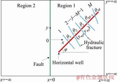
Figure 1 Schematic of FCMFH well in LC gas reservoir with a fault

1) Each reservoir region (i.e., Region 1 or Region 2) is homogeneous and isotropic reservoir, but the two regions can have different properties (e.g., porosity, permeability, and rock compressibility). The properties of both the two regions are independent of pressure.

2) The gas reservoir, which has a uniform thickness for Region 1 and Region 2, is bounded by upper and lower impermeable layers. The fault is assumed to be located at x=0 and infinitely extended along the y-axis. The fault is considered as a partially communicating interface, where flux is continuous and pressure can be discontinuous. The orientation of the horizontal well can be arbitrary direction, and the angle between the horizontal well and x-axis is set as φ.

3) Hydraulic fractures completely vertically penetrate the gas reservoir, and the number of hydraulic fractures is assumed to be M. Each hydraulic fracture symmetrically distributes about the horizontal well and can intersect with the horizontal well with any angle (e.g., θ_j for the jth hydraulic fracture). The coordinates of the intersection between the jth hydraulic fracture and horizontal well are set to be (x_wj, y_wj). Gas flow within each finite-conductivity hydraulic fracture is viewed as an incompressible linear flow.

4) Gas flow in LC gas reservoirs is assumed to be isothermal single-phase flow, which follows the Darcy law. Initial reservoir pressure is uniformly distributed in Region 1 and Region 2.

3 Mathematical models

3.1 Seepage model for LC gas reservoirs

If a point source is assumed to be located at coordinates (x_w, y_w) in Region 1 and gas is withdrawn from the point source with flow rate q_sc(t), gas flow in the LC gas reservoir can be described by the following governing equations (Appendix A):

                     (1)

 (2)

where subscripts 1 and 2 represent Region 1 and Region 2, respectively; k is the permeability, m²; μ is the gas viscosity, Pa·s; p is the reservoir pressure, Pa; Z is the deviation factor of natural gas; x and y are the coordinates, m; p_sc is the pressure at standard condition, Pa; T is the gas reservoir temperature, K; q_sc is the production rate of the point source at standard condition, m³/s; T_sc is the temperature at standard condition, K; h is the reservoir thickness, m; δ is Dirac delta function; x_w, y_w are the coordinates of the point source, m; f is the porosity; C_t is the total compressibility, Pa^-1; t is the time, s.

In order to linearize Eqs. (1) and (2), the pseud-pressure is introduced as:

              (3)

Substituting Eq. (3) into Eqs. (1) and (2), one can derive that:

                    (4)

          (5)

Gas viscosity μ in both Eqs. (4) and (5) is the function of pressure, which is usually estimated at the initial reservoir pressure, i.e., μ=μ(p_i)=μ_i. Then, Eqs. (4) and (5) become respectively:

                   (6)

         (7)

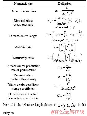
Introducing dimensionless variables (see Table 1), Eqs. (6) and (7) are rewritten as, respectively:

                       (8)

             (9)

Table 1 Definitions of dimensionless variables for FCMFH wells in LC gas reservoirs

Dimensionless outer boundary conditions

 (10)

 (11)

Dimensionless interface boundary conditions

 (12)

                  (13)

where λ is the mobility ratio defined in Table 1; S_F is the skin factor across the fault.

Dimensionless initial conditions

   (14)

Taking Laplace transform of Eqs. (8)-(14) with respect to (w.r.t.) t_D and infinite Fourier transform w.r.t. y_D respectively, the Laplace-space point source solution for LC gas reservoirs is able to be derived as (Appendix B):

 (15)

where

                             (16)

                             (17)

                (18)

Based on superposition principle in Laplace space [35, 36], pressure response at arbitrary position in Region 1 caused by an MFH well is obtained by integrating Eq. (15) along the line segments of all hydraulic fractures:

                         (19)

where M is the number of hydraulic fractures; θ_j is the angle between the jth hydraulic fracture and horizontal well, (°); φ is the angle between the horizontal well and x-axis, (°); L_fDj is the dimensionless half-length of the jth hydraulic fracture; q_fD is the dimensionless fracture flux density; x_wDj and y_wDj are the dimensionless coordinates of the intersection between the jth hydraulic fracture and horizontal well.

3.2 Seepage model for hydraulic fractures

Gas flow within each finite-conductivity hydraulic fracture of FCMFH wells is usually viewed as an incompressible linear flow. The seepage model of gas flow within the jth hydraulic fracture is established based on coordinate system (x_j, y_j) (see Figure 2) (Appendix C):

Figure 2 Relationship diagram of different coordinate systems

          (20)

 (21)

 (22)

Equations (20)-(22) can be used to obtain the pressure at any position within the hydraulic fractures, which is expressed as follows:

              (23)

for ;

               (24)

for , where ψ_wDH is the dimensionless wellbore pseud-pressure.

3.3 Semi-analytical model of an FCMFH well in LC gas reservoirs

The solution for gas flow in LC gas reservoirs (i.e., Eq. (19)) can be combined with the solution for gas flow in hydraulic fracture (i.e., Eqs. (23) and (24)) by the following expression:

 (25)

where and .

Substituting Eq. (25) into Eqs. (23) and (24) and taking the Laplace transform w.r.t. t_D, one can derive that:

                (26)

for ;

                (27)

for , where is presented in Eq. (19).

The production rate of the FCMFH well is the sum of the flow rates from all the hydraulic fractures, which is expressed as:

                   (28)

Introducing the dimensionless variables (as shown in Table 1) and taking the Laplace transform w.r.t. t_D, Eq. (28) can be rewritten as:

                 (29)

Equations (26), (27) and (29) associating with Eq. (19) form a mathematical model of an FCMFH well in LC reservoirs in Laplace space. However, the proposed model is difficult to be analytically solved, and thus fracture discrete method is used to derive the semi-analytical solution. Each of hydraulic fractures is discretized into several segments. As shown in Figure 3, the two wings of the jth hydraulic fracture are discretized into N_j segments with the same length, respectively, and thus the total number of segments for an FCMFH well is . The flux is uniformly distributed in each segment. The mid-point coordinates of the ith segment of the jth hydraulic fracture, (x_mi,j, y_mi,j), are

,

                  (30)

             (31)

where is the fracture-segment length of the jth hydraulic fracture, m.

The coordinates (x_mi,j, y_mi,j) are transformed into the dimensionless form as follows:

,

                  (32)

,

             (33)

where x_mDi,j=x_mi,j/L, y_mDi,j=y_mi,j/L, x_wDj=x_wj/L, y_wDj= y_wj/L, and △L_fDj=△L_fj/L.

The distance between the coordinates (x_wj, y_wj) and the coordinates (x_wj+1, y_wj+1) is defined as:

Figure 3 Discretization diagram of jth hydraulic fracture

,

                   (34)

If hydraulic fractures are discretized, Eqs. (26), (27) and (29) associating with Eq. (19) can be rewritten in the discrete form:

,

                  (35)

             (36)

                 (37)

where q_fDi,j is the dimensionless fracture flux density of the ith segment of the jth hydraulic fracture; is given as:

   (38)

Equations (35)-(38) consist of linear equations with unknowns, i.e., andBy solving the linear equations, the dimensionless wellbore pseud-pressure in Laplace space is obtained. To incorporate the impact of the wellbore storage and skin, Duhamel’s principle is used as follows [37, 38]:

           (39)

where S is the skin factor near the wellbore; C_D is the dimensionless wellbore storage coefficient defined in Table 1. Finally, the numerical Laplace inversion method [39] is employed to transform the Laplace-space pseud-pressure to the real-space pseud-pressure

4 Model validation

The proposed semi-analytical model is validated by comparing with numerical results generated by the Saphir numerical simulator in this section. The schematic of the numerical model is shown in Figure 4, from which it is seen that an FCMFH well is located in Region 1 of an LC gas reservoir separated by a fault. The dimensionless size of the LC gas reservoir is set as a large value (i.e., 4000×4000), which could avoid the boundary effect within the simulation time. The unstructured grid system (i.e., Voronoi grid), which is automatically generated by the Saphir numerical simulator, is applied to the spatial discretization of the numerical model (see Figure 5). The input parameters used for numerical simulations are mainly collected from the published literature [40] and are listed in Table 2. Figure 6 shows the comparison of the results obtained by the proposed model and Saphir numerical simulator. It is seen that the proposed solution agrees excellently with Saphir numerical solution, demonstrating that the proposed semi-analytical model is able to be used to investigate the pressure characteristics of an FCMFH well in LC gas reservoirs with a fault.

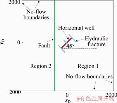
Figure 4 Schematic of an FCMFH well in an LC gas reservoir with a fault

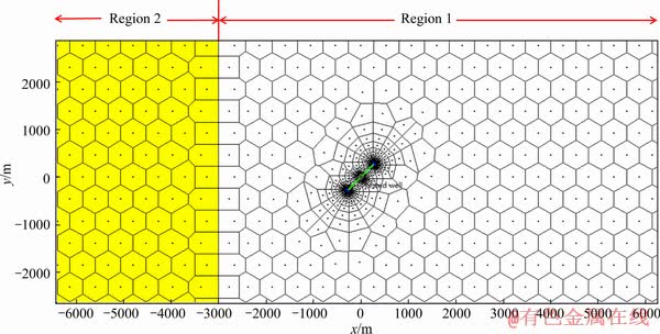
Figure 5 Local spatial discretization of numerical model of an FCMFH well in an LC gas reservoir with a fault by using Saphir numerical simulator

Table 2 Basic data for numerical simulations

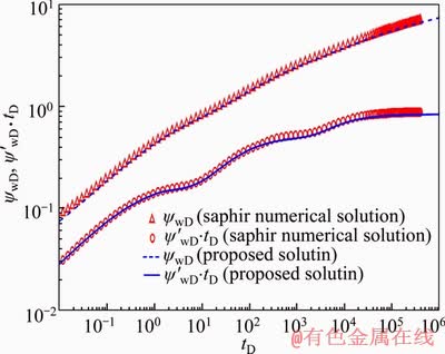
Figure 6 Comparison of results obtained by proposed model and Saphir numerical simulator (M=3, L_fj=40 m, S=0, C_D=0, C_fD=20, θ_j=90°, φ=45°, η=1, λ=0.2, S_F=0, x_w=3000 m, y_w=0 m, △y_w=△y_w1=△y_w2=400 m)

5 Type curves and sensitivity analysis

The proposed model is employed to obtain the dimensionless wellbore pseud-pressure (DWPP) and dimensionless wellbore pseud-pressure derivative (DWPPD) of an FCMFH well in LC gas reservoirs. Type curve of an FCMFH well in LC gas reservoirs is plotted to study the characteristics of transient pressure responses and identify flow regimes. The effects of some parameters on the DWPP and DWPPD responses are analyzed in detail.

5.1 Type curves

Figure 7 shows type curve of an FCMFH well in LC gas reservoirs with a fault. Type curve consists of the DWPP curve (i.e., ψ_wD versus t_D/C_D curve) and the DWPPD curve (i.e., versus t_D/C_D curve). It is observed from Figure 7 that the type curve can be divided into nine parts, which correspond to nine flow regimes as follows:

Figure 7 Type curve of an FCMFH well in LC gas reservoirs with a fault (M=3, L_fj=40 m, S=10^-3, C_D=10^-6, C_fD=20, θ_j=90°, φ=45°, η=1, λ=0.2, S_F=1000, x_w=3000 m, y_w=0 m, △y_w=△y_w1=△y_w2=400 m)

1) Wellbore storage flow period (WSFP): DWPP curve and DWPPD curve show the same straight line with unit slope. During the WSFP, the produced gas is all from the wellbore-storage gas, and the gas in the reservoir has not entered into the wellbore.

2) Transitional flow period after WSFP (TFP-WSFP): DWPPD curve exhibits a “hump”, which is mainly affected by the seepage capability near the wellbore. During this period, the gas in the reservoir begins to flow into the wellbore, and the pressure wave travels in the reservoir area near the wellbore.

3) Bilinear flow period (BFP): DWPPD curve exhibits a 0.25-slope straight line. During the BFP, the two linear flows take place together: one is within the hydraulic fracture; the other is perpendicular to the reservoir-fracture contact surface (see Figure 8(a)).

4) First linear flow period (FLFP): DWPPD curve shows a 0.5-slope straight line. During the FLFP, the linear flow perpendicular to the reservoir-fracture contact surface takes place, and the linear flow of each hydraulic fracture cannot interact with each other (see Figure 8(b)).

5) First pseudo-radial flow period (FPRFP): DWPPD curve exhibits a horizontal line. During the FPRFP, the pseudo-radial flow independently takes place around each of hydraulic fractures (see Figure 8(c)).

6) Second linear flow period (SLFP): DWPPD curve exhibits a straight line with a 0.5 slope. In the SLFP, pressure waves caused by adjacent hydraulic fractures have interacted with each other, and a linear flow occurs along the direction of hydraulic fractures (see Figure 8(d)).

7) Second pseudo-radial flow period (SPRFP): DWPPD curve shows a horizontal line with the magnitude being 0.5. During the SPRFP, the pseudo-radial flow toward the FCMFH well occurs in Region 1 and the pressure wave has not reached the fault (see Figure 8(e)).

8) Transitional flow period after SPRFP (TFP-SPRFP): DWPPD curve appears as a step. During the TFP-SPRFP, the pressure wave has arrived at the fault but has not transmitted into Region 2 totally. The flow period is mainly affected by the properties of the fault and Region 2, which will be analyzed in detail later.

9) Third pseudo-radial flow period (TPRFP): DWPPD curve shows a horizontal line with a constant value, whose magnitude is dependent on the properties of Region 2. During the TPRFP, the pressure wave has totally transmitted into Region 2 and the pseudo-radial flow toward the FCMFH well takes place in the whole gas reservoir including Region 1 and Region 2 (see Figure 8(f)).

It should be noted that not all the flow regimes described above exist for FCMFH wells in LC gas reservoirs with a fault. Depending on the reservoir/well properties, some of these flow regimes may be absent. Therefore, sensitivity analysis will be conducted in the next subsection to study the effect of some parameters on the pressure behaviors.

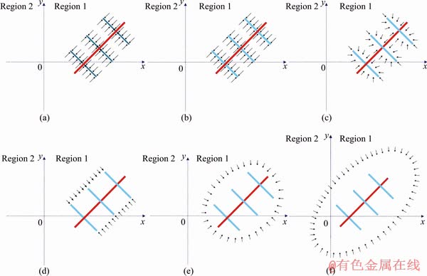
Figure 8 Flow pattern of an FCMFH well in LC gas reservoirs with a fault

5.2 Sensitivity analysis

Figure 9 shows the effect of skin factor across the fault (S_F) on the DWPP and DWPPD responses of an FCMFH well in LC gas reservoirs with a fault, from which it is seen that the S_F merely affects the flow periods after the pressure wave has arrived at the fault, i.e., TFP-SPRFP and TPRFP. Increasing the S_F will result in a longer duration of the TFP-SPRFP and a later start time of the TPRFP. The reason of this phenomenon is that a larger S_F represents a larger flow resistance across the fault. If the flow resistance across the fault increases, the drawdown pressure should be enhanced to keep the production rate unchanged, and the transmission time of the pressure wave across the fault should become longer.

Figure 9 Effect of skin factor across fault (S_F) on type curve of an FCMFH well in LC gas reservoirs with a fault (M=3, L_fj=40 m, S=10^-3, C_D=10^-6, C_fD=20, θ_j=90°, φ=45°, η=1, λ=1, x_w=3000 m, y_w=0 m, △y_w=△y_w1= △y_w2=400 m)

Figure 10 shows the effect of the distance between the horizontal well center and the fault (x_w) on the DWPP and DWPPD responses of an FCMFH well in LC gas reservoirs with a fault. It is observed that the x_w affects the duration of the SPRFP and the start time of the TFP-SPRFP. The smaller the x_w is, the shorter the duration of the SPRFP is and the earlier the start time of the TFP-SPRFP becomes. It is noted that if the FCMFH well is located near the fault, the SPRFP may disappear. The reason is that as the x_w becomes smaller, the pressure wave reaches the fault earlier.

Figure 11 shows the effect of mobility ratio (λ) on the DWPP and DWPPD responses of an FCMFH well in LC gas reservoirs with a fault. Based on the definition of the λ (as shown in Table 1), the λ represents the flow capability of Region 2 compared with Region 1. The flow capability of Region 2 increases with increasing λ. It is clear from Figure 11 that λ has an impact on pressure responses of FCMFH wells after the pressure wave reaches the fault, and the DWPP and DWPPD increase with decreasing λ. The cause of this phenomenon is that the decrease of λ reduces the flow capability of Region 2, and thus the drawdown pressure should be enhanced to keep the production rate unchanged.

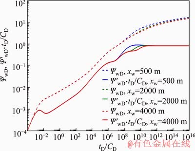
Figure 10 Effect of distance between horizontal well center and fault (x_w) on type curve of an FCMFH well in LC gas reservoirs with a fault (M=3, L_fj=40 m, S=10^-3, C_D=10^-6, C_fD=20, θ_j=90°, φ=45°, η=1, λ=0.2, S_F=1000, y_w=0 m, △y_w=△y_w1=△y_w2=400 m)

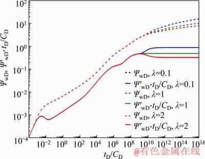
Figure 11 Effect of mobility ratio (λ) on type curve of an FCMFH well in LC gas reservoirs with a fault (M=3, L_fj=40 m, S=10^-3, C_D=10^-6, C_fD=20, θ_j=90°, φ=45°, η=1, S_F=0, x_w=3000 m, y_w=0 m, △y_w=△y_w1=△y_w2=400 m)

Figure 12 shows the effect of diffusivity ratio (η) on the DWPP and DWPPD responses of an FCMFH well in LC gas reservoirs with a fault. According to the definition of η (see Table 1), η is inversely proportional to under the same other parameters (e.g., the same λ). The storage capability of Region 2 increases with decreasing η. It is seen from Figure 12 that η mainly has an impact on the TFP-SPRFP, where the DWPP and DWPPD decrease with decreasing η. The reason is that decreasing η improves the storage capability of Region 2, and thus the drawdown pressure must decrease to maintain the fixed production rate.

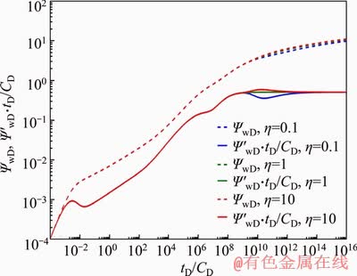
Figure 12 Effect of diffusivity ratio (η) on type curve of an FCMFH well in LC gas reservoirs with a fault (M=3, L_fj=40 m, S=10^-3, C_D=10^-6, C_fD=20, θ_j=90°, φ=45°, λ=1, S_F=0, x_w=3000 m, y_w=0 m, △y_w=△y_w1=△y_w2=400 m)

Figure 13 shows the effect of dimensionless fracture conductivity coefficient (C_fD) on the DWPP and DWPPD responses of an FCMFH well in LC gas reservoirs with a fault. It is clear that C_fD primarily affects the early-time flow periods including TFP-WSFP, BFP, and FLFP. As C_fD increases, the DWPP and DWPPD decrease, the BFP lasts shorter, and the FLFP appears earlier. The reason is that increasing C_fD causes the increase of the hydraulic-fracture permeability; in other words, increasing C_fD leads to the improvement of the seepage capability near the wellbore. Therefore, in order to keep the production rate constant, the drawdown pressure of the FCMFH well should decrease with increasing C_fD. Furthermore, with the improvement of the hydraulic-fracture permeability,the BFP lasts shorter and then the FLFP begins earlier.

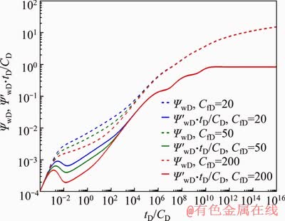
Figure 13 Effect of dimensionless fracture conductivity coefficient (C_fD) on type curve of an FCMFH well in LC gas reservoirs with a fault (M=3, L_fj=40 m, S=10^-3, C_D=10^-6, θ_j=90°, φ=45°, η=1, λ=0.2, S_F=1000, x_w=3000 m, y_w=0 m, △y_w=△y_w1=△y_w2=400 m)

Figure 14 shows the effect of fracture spacing (△y_w) on the DWPP and DWPPD responses of an FCMFH well in LC gas reservoirs with a fault. It is obvious that △y_w has an effect on the flow periods from FPRFP to SPRFP. As △y_w decreases, the duration of the FPRFP gets shorter, and the SLFP and SPRFP begin earlier. If △y_w is small enough, the FPRFP may be masked by the SLFP and SPRFP. This is because that as △y_w decreases, the interference between adjacent hydraulic fractures occurs earlier.

It is noted that some differences are observed at some intermediate-time flow periods in Figures 9, 10, 12 and 14. The explanations are given as follows: S_F only has an effect on the TFP-SPRFP and TPRFP (as shown in Figure 9); x_w mainly affects the SPRFP and TFP-SPRFP (as shown in Figure 10); η mainly has an impact on the TFP-SPRFP (as shown in Figure 12); △y_w mainly has an effect on the FPRFP, SLFP, and SPRFP (as shown in Figure 14).

Figure 14 Effect of fracture spacing (△y_w) on type curve of an FCMFH well in LC gas reservoirs with a fault (M=3, L_fj=40 m, S=10^-3, C_D=10^-6, C_fD=20, θ_j=90°, φ=45°, η=1, λ=0.2, S_F=1000, x_w=3000 m, y_w=0 m, △y_w= △y_w1=△y_w2)

Figure 15 shows the effect of the number of hydraulic fractures (M) on the DWPP and DWPPD responses of an FCMFH well in LC gas reservoirs with a fault. It is clear that M mainly has an impact on the flow periods (i.e., from TFP-WSFP to SPRFP) that the pressure wave has not reached the fault. As M increases, the DWPP and DWPPD decrease. The reason is that increasing M means the improvement of the seepage capability near the wellbore, and thus the drawdown pressure of FCMFH wells with a fixed production rate should decrease with increasing M.

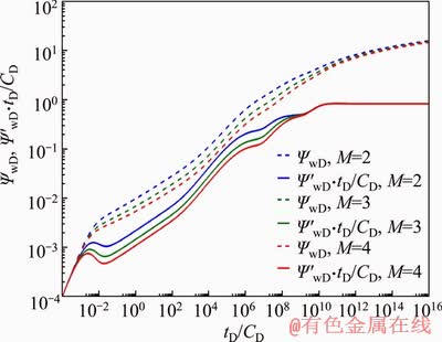
Figure 15 Effect of number of hydraulic fractures (M) on type curve of an FCMFH well in LC gas reservoirs with a fault (L_fj=40 m, S=10^-3, C_D=10^-6, C_fD=20, θ_j=90°, φ=45°, η=1, λ=0.2, S_F=1000, x_w=3000 m, y_w=0 m, △y_w=△y_wj=400 m)

6 Conclusions

1) A semi-analytical model of FCMFH wells in LC gas reservoirs is proposed based on Laplace-space superposition principle and fracture discrete method. The proposed model is validated against the results obtained by Saphir numerical simulator.

2) Type curves of an FCMFH well in LC gas reservoirs are obtained to conduct the pressure transient analysis based on the established model. It is found that there are nine possible flow regimes in the whole production process of the FCMFH well. Before the pressure wave reaches the fault, the first seven flow periods (i.e., from WSFP to SPRFP) appear one after another; after the pressure wave arrives at the fault, the last two flow periods (i.e., TFP-SPRFP and TPRFP) just turn up.

3) The effects of some parameters on type curves and flow regimes are discussed in detail. It is found that dimensionless fracture conductivity coefficient, fracture spacing, and number of hydraulic fractures mainly affect the pressure behaviors before the pressure wave reaches the fault; skin factor across the fault, mobility ratio, and diffusivity ratio only have an impact on the pressure behaviors after the pressure wave arrives at the fault.

4) The proposed model provides an efficient method to obtain pressure responses of FCMFH wells in LC gas reservoirs. It is also helpful to further develop analytical/semi-analytical models for other complex well types in LC gas reservoirs.

Appendix A Derivation of governing equations for point source in LC gas reservoirs

Based on mass conservation, continuity equations for LC gas reservoirs with a point source located at (x_w, y_w) are given as:

                     (A1)

       (A2)

where subscript 1 and 2 represent Region 1 and Region 2, respectively; ρ is the gas density, kg/m³; υ_x is the x-direction gas velocity, m/s; υ_y is the y-direction gas velocity, m/s; ρ_sc is the gas density at standard condition, kg/m³; q_sc is the production rate of the point source at standard condition, m³/s; h is the reservoir thickness, m; δ is Dirac delta function; x, y are the coordinates, m; x_w, y_w are the coordinates of the point source, m; f is the porosity; t is the time, s.

According to the Darcy law, the gas velocities in the x and y directions are described by, respectively:

                           (A3)

                           (A4)

where subscript j=1, 2 represents Region 1 and Region 2, respectively; k is the permeability, m²; μ is the gas viscosity, Pa·s; p is the reservoir pressure, Pa.

The equation of state for real gas is given as follows:

                            (A5)

where subscript j=1, 2 represents Region 1 and Region 2, respectively; M_g is the gas molar mass, kg/mol; Z is the deviation factor of natural gas; R is the universal gas constant, J/(mol·K); T is the gas reservoir temperature, K.

The gas compressibility and rock compressibility are defined, respectively, as:

                         (A6)

                            (A7)

where subscript j=1, 2 represents Region 1 and Region 2, respectively; C_g is the gas compressibility, Pa^-1; C_r is the rock compressibility, Pa^-1.

Substituting Eqs. (A3)-(A7) into Eqs. (A1) and (A2) yields that:

                  (A8)

 (A9)

where C_t1 and C_t2 are the total compressibility of Region 1 and Region 2, respectively, which are defined by C_tj=C_g+C_rj, j=1, 2. It is noted that C_t1 and C_t2 are actually the functions of pressure, but they are usually treated as constants for engineering applications, i.e., C_t1=C_t1(p_i) and C_t2=C_t2(p_i).

Appendix B Derivation of Laplace-space point source solution for LC gas reservoirs

1) Laplace transform of Eqs. (8)-(14) w.r.t. t_D

                      (B1)

             (B2)

  (B3)

 (B4)

   (B5)

                   (B6)

where s is the Laplace transform variable; , andare the corresponding Laplace-space variables of ψ_1D, ψ_2D and q_D, respectively, which are given as:

     (B7)

    (B8)

                 (B9)

2) Infinite Fourier transform of Eqs. (B1)-(B6) w.r.t. y_D

,

x_D>0                             (B10)

           (B11)

  (B12)

    (B13)

                   (B14)

where ω is the Fourier transform variable;and are the corresponding Fourier-space variables ofandrespectively, which are defined as:

    (B15)

     (B16)

Equations (B10)-(B14) consist of ordinary differential equations w.r.t. x_D, which are able to be analytically solved as follows:

                     (B17)

     (B18)

where

                            (B19)

                           (B20)

              (B21)

3) Inverse Fourier transform of Eq. (B17) w.r.t. ω

      (B22)

Equation (B22) is obtained based on the expression of inverse Fourier transform:

   (B23)

It is obvious that the integrand in Eq. (B22) is the product of two parts (i.e., A₁ and A₂):

           (B24)

        (B25)

Equation (B25) can be rewritten as the sum of two parts:

                          (B26)

where

           (B27)

          (B28)

It is noted that A₁ in Eq. (B24) and A₂₁ in Eq. (B27) are even functions of ω, A₂₂ in Eq. (B28) is odd function of ω.

Considering the odevity of functions and the symmetry of integral domain, Eq. (B22) can be simplified as:

          (B29)

Appendix C Derivation of dimensionless model for gas flow within a hydraulic fracture

Because of a very small volume within hydraulic fracture compared with the reservoir volume, gas flow within hydraulic fractures is usually viewed as an incompressible linear flow. To study the linear flow within hydraulic fractures, the coordinate system for the jth hydraulic fracture is employed to establish the dimensionless model for gas flow within the jth hydraulic fracture (see Figure 2). The governing equation of gas flow within the jth hydraulic fracture can be described as [41]:

(C1)

where L_fj is the half-length of the jth hydraulic fracture, m; w_f is the hydraulic fracture width, m; p_f is the pressure in hydraulic fractures, Pa.

Introducing the pseud-pressure:

                    (C2)

Equation (C1) becomes:

  (C3)

The fracture flux density of the jth hydraulic fracture is described by:

                 (C4)

where and q_f is the fracture flux density at standard condition, m²/s.

Considering the incompressible linear flow within hydraulic fractures, the wellbore conditions can be described as:

                    (C5)

                      (C6)

where k_f is the permeability of hydraulic fracture, m².

The boundary conditions of the reservoir-fracture contact surface can be described based on the mass conservation:

 (C7)

             (C8)

Owing to the hydraulic fracture width being very small, the y_j-direction pressure variation within the jth hydraulic fracture is usually neglected, and the y_j-direction average pressure is introduced as:

 (C9)

With the aid of Eqs. (C7)-(C9), Eq. (C3) can be rewritten as:

             (C10)

Substituting Eq. (C4) into Eq. (C10) yields that:

          (C11)

Based on Eq. (C9), Eqs. (C5) and (C6) can be rewritten as:

 (C12)

   (C13)

Considering the dimensionless variables (see Table 1), Eqs. (C11)-(C13) are rewritten in dimensionless form:

         (C14)

 (C15)

 (C16)

References

[1] YAXLEY L M. Effect of a partially communicating fault on transient pressure behavior [J]. SPE Formation Evaluation, 1987, 2(4): 590-598. DOI: 10.2118/14311- PA.

[2] MOLINA O M, ZEIDOUNI M. Analytical model to detect fault permeability alteration induced by fault reactivation in compartmentalized reservoirs [J]. Water Resources Research, 2018, 54(8): 5841-5855. DOI: 10.1029/2018WR022872.

[3] SU K, LIAO X, ZHAO X. Transient pressure analysis and interpretation for analytical composite model of CO₂ flooding [J]. Journal of Petroleum Science and Engineering, 2015, 125: 128-135. DOI: 10.1016/j.petrol.2014.11.007.

[4] ZHANG W, CUI Y, JIANG R, XU J, QIAO X, JIANG Y, ZHANG H, WANG X. Production performance analysis for horizontal wells in gas condensate reservoir using three- region model [J]. Journal of Natural Gas Science and Engineering, 2019, 61: 226-236. DOI: 10.1016/j.jngse.2018. 11.004.

[5] DENG Q, NIE R S, JIA Y L, GUO Q, JIANG K J, CHEN X, LIU B H, DONG X F. Pressure transient behavior of a fractured well in multi-region composite reservoirs [J]. Journal of Petroleum Science and Engineering, 2017, 158: 535-553. DOI: 10.1016/j.petrol.2017.08.079.

[6] WANG Y, YI X. Transient pressure behavior of a fractured vertical well with a finite-conductivity fracture in triple media carbonate reservoir [J]. Journal of Porous Media, 2017, 20(8): 707-722. DOI: 10.1615/JPorMedia.v2018.30.

[7] REN J, GUO P. Nonlinear seepage model for multiple fractured horizontal wells with the effect of the quadratic gradient term [J]. Journal of Porous Media, 2018, 21(3): 223-239. DOI: 10.1615/JPorMedia.v21.i3.30.

[8] WEI M Q, DUAN Y G, CHEN W, FANG Q T, LI Z L, GUO X R. Blasingame production decline type curves for analysing a multi-fractured horizontal well in tight gas reservoirs [J]. Journal of Central South University, 2017, 24(2): 394-401. DOI: 10.1007/s11771-017-3441-9.

[9] WANG J, JIA A, WEI Y, QI Y. Approximate semi-analytical modeling of transient behavior of horizontal well intercepted by multiple pressure-dependent conductivity fractures in pressure-sensitive reservoir [J]. Journal of Petroleum Science and Engineering, 2017, 153: 157-177. DOI: 10.1016/j.petrol. 2017.03.032.

[10] LI Z, DUAN Y, WEI M, PENG Y, CHEN Q. Pressure performance of interlaced fracture networks in shale gas reservoirs with consideration of induced fractures [J]. Journal of Petroleum Science and Engineering, 2019, 178: 294-310. DOI: 10.1016/j.petrol.2019.03.048.

[11] REN J, GUO P. A general analytical method for transient flow rate with the stress-sensitive effect [J]. Journal of Hydrology, 2018, 565: 262-275. DOI: 10.1016/j.jhydrol. 2018.08.019.

[12] REN J, ZHENG Q, ZHAO C. A modified Blasingame production analysis method for vertical wells considering the quadratic gradient term [J]. Energies, 2019, 12: 2092. DOI: 10.3390/en12112092.

[13] ZHAO C B, HOBBS B, ORD A. Finite element modeling of convective pore-fluid flow in fluid-saturated porous rocks within upper crust: An overview [J]. Journal of Central South University, 2019, 26(3): 501-514. DOI: 10.1007/s11771- 019-4022-x.

[14] LIN H, DENG J G, LIU W, XIE T, XU J, LIU H L. Numerical simulation of hydraulic fracture propagation in weakly consolidated sandstone reservoirs [J]. Journal of Central South University, 2018, 25(12): 2944-2952. DOI: 10.1007/s11771-018-3964-8.

[15] REN J, ZHENG Q, GUO P, PENG S, WANG Z, DU J. Pore-scale lattice Boltzmann simulation of two-component shale gas flow [J]. Journal of Natural Gas Science and Engineering, 2019, 61: 46-70. DOI: 10.1016/j.jngse.2018. 11.011.

[16] BIXEL H C, LARKIN B K, van POOLLEN H K. Effect of linear discontinuities on pressure build-up and drawdown behavior [J]. Journal of Petroleum Technology, 1963, 15(8): 885-895. DOI: https://doi.org/10.2118/611-PA.

[17] AMBASTHA A K, MCLEROY P G, GRADER A S. Effects of a partially communicating fault in a composite reservoir on transient pressure testing [J]. SPE Formation Evaluation, 1989, 4(2): 210-218. DOI: 10.2118/16764-PA.

[18] BOURGEOIS M J, DAVIAU F H, BOUTAUD DE LA COMBE J L. Pressure behavior in finite channel-levee complexes [J]. SPE Formation Evaluation, 1996, 11(3): 177-184. DOI: 10.2118/26461-PA.

[19] KUCHUK F J, HABASHY T. Pressure behavior of laterally composite reservoirs [J]. SPE Formation Evaluation, 1997, 12(1): 47-56. DOI: 10.2118/24678-PA.

[20] ANDERSON E I. Analytical solutions for flow to a well through a fault [J]. Advances in Water Resources, 2006, 29(12): 1790-1803. DOI: 10.1016/j.advwatres.2005.12.010.

[21] EZULIKE O, IGBOKOYI A. Horizontal well pressure transient analysis in anisotropic composite reservoirs—A three dimensional semi-analytical approach [J]. Journal of Petroleum Science and Engineering, 2012, 96-97: 120-139. DOI: 10.1016/j.petrol.2012.09.002.

[22] ZEIDOUNI M. Analytical model of leakage through fault to overlying formations [J]. Water Resources Research, 2012, 48: W00N02. DOI: 10.1029/2012WR012582.

[23] ZEIDOUNI M. Semi-analytical model of pressure perturbations induced by fault leakage in multilayer system [J]. Journal of Hydrologic Engineering, 2016, 21(6): 04016011. DOI: 10.1061/(ASCE)HE.1943-5584.0001359.

[24] FENG G Q, LIU Q G, ZHANG L H, ZENG Y. Pressure transient behavior analysis in a dual-porosity reservoir with partially communicating faults [J]. Journal of Natural Gas Science and Engineering, 2016, 32: 373-379. DOI: 10.1016/j.jngse.2016.04.046.

[25] LUO W J, TANG C F, WANG X D. Pressure transient analysis of a horizontal well intercepted by multiple non-planar vertical fractures [J]. Journal of Petroleum Science and Engineering, 2014, 124: 232-242. DOI: 10.1016/j.petrol.2014.10.002.

[26] REN J, GUO P. A novel semi-analytical model for finite- conductivity multiple fractured horizontal wells in shale gas reservoirs [J]. Journal of Natural Gas Science and Engineering, 2015, 24: 35-51. DOI: 10.1016/j.jngse.2015.03. 015.

[27] WANG Y, YI X. Flow modeling of well test analysis for a multiple-fractured horizontal well in triple media carbonate reservoir [J]. International Journal of Nonlinear Sciences and Numerical Simulation, 2018, 19(5): 439-457. DOI: 10.1515/ijnsns-2016-0075.

[28] GU D, DING D, GAO Z, TIAN L, LIU L, XIAO C. A fractally fractional diffusion model of composite dual-porosity for multiple fractured horizontal wells with stimulated reservoir volume in tight gas reservoirs [J]. Journal of Petroleum Science and Engineering, 2019, 173: 53-68. DOI: 10.1016/j.petrol.2018.10.011.

[29] REN J, GUO P. Nonlinear flow model of multiple fractured horizontal wells with stimulated reservoir volume including the quadratic gradient term [J]. Journal of Hydrology, 2017, 554: 155-172. DOI: 10.1016/j.jhydrol.2017.09.005.

[30] REN J, GUO P, PENG S, MA Z. Performance of multi-stage fractured horizontal wells with stimulated reservoir volume in tight gas reservoirs considering anomalous diffusion [J]. Environmental Earth Sciences, 2018, 77(22): 768. DOI: 10.1007/s12665-018-7947-8.

[31] OZKAN E, BROWN M L, RAGHAVAN R, KAZEMI H. Comparison of fractured-horizontal-well performance in tight sand and shale reservoirs [J]. SPE Reservoir Evaluation and Engineering, 2011, 14(2): 248-259. DOI: 10.2118/121290-PA.

[32] STALGOROVA E, MATTAR L. Analytical model for history matching and forecasting production in multifrac composite systems [C]// SPE Canadian Unconventional Resources Conference. Calgary: Society of Petroleum Engineers, 2012: 1-17. DOI: 10.2118/162516-MS.

[33] TIAN L, XIAO C, LIU M, GU D, SONG G, CAO H, LI X. Well testing model for multi-fractured horizontal well for shale gas reservoirs with consideration of dual diffusion in matrix [J]. Journal of Natural Gas Science and Engineering, 2014, 21: 283-295. DOI: 10.1016/j.jngse.2014.08.001.

[34] ZENG J, WANG X, GUO J, ZENG F, ZHANG Q. Composite linear flow model for multi-fractured horizontal wells in tight sand reservoirs with the threshold pressure gradient [J]. Journal of Petroleum Science and Engineering, 2018, 165: 890-912. DOI: 10.1016/j.petrol.2017.12.095.

[35] OZKAN E. Performance of horizontal wells [D]. Tulsa: University of Tulsa, 1988. http://pqdt.calis.edu.cn/Detail. aspx?pid=HWfJ6%2fs7KC0%3d.

[36] TANG X, CHEN Z, CHU H, LIAO X, CHEN H, ZHANG J. Well testing interpretation for horizontal well with hydraulic fractures and interconnected micro-fractures [J]. Journal of Petroleum Science and Engineering, 2019, 179: 546-557. DOI: 10.1016/j.petrol.2019.04.074.

[37] VAN EVERDINGEN A F, HURST W. The application of the Laplace transformation to flow problems in reservoirs [J]. Journal of Petroleum Technology, 1949, 1(12): 305-324. DOI: https://doi.org/10.2118/949305-G.

[38] HUANG S, DING G, WU Y, HUANG H, LAN X, ZHANG J. A semi-analytical model to evaluate productivity of shale gas wells with complex fracture networks [J]. Journal of Natural Gas Science and Engineering, 2018, 50: 374-383. DOI: 10.1016/j.jngse.2017.09.010.

[39] STEHFEST H. Numerical inversion of Laplace transforms [J]. Communications of the ACM, 1970, 13: 47-49. https:// dl.acm.org/citation.cfm?id=361969.

[40] CHOO Y K, WU C H. Transient pressure behavior of multiple-fractured gas wells [C]// Low Permeability Reservoirs Symposium. Denver, Colorado, USA: Society of Petroleum Engineers, 1987: 73-89. DOI: https://doi.org/ 10.2118/16398-MS.

[41] CINCO L H, SAMANIEGO V F, DOMINGUEZ A N. Transient pressure behavior for a well with a finite-conductivity vertical fracture [J]. Society of Petroleum Engineers Journal, 1978, 18(4): 253-264. DOI: https://doi.org/10.2118/6014-PA.

(Edited by FANG Jing-hua)

中文导读

线性复合气藏有限导流多段压裂水平井压力动态分析

摘要：断块气藏是一种在现实中非常常见的气藏，该类气藏被一些线性滤失断层分割成多个具有不同物性的储层区域，这类气藏也被称为线性复合气藏。虽然目前已有一些解析/半解析模型用于研究线性复合气藏中生产井的压力动态，但是大部分成果针对直井，而对多段压裂水平井研究得较少。当压力波传播到滤失断层后，多段压裂水平井的压力动态将会受到滤失断层的影响，因此，弄清楚滤失断层对多段压裂水平井压力动态的影响对开发断块气藏非常重要。基于Laplace空间的叠加原理和裂缝离散方法，本文建立了线性复合气藏有限导流多段压裂水平井的半解析模型。通过与商业数值模拟器进行结果对比，检验了该模型的可靠性。绘制了线性复合气藏中有限导流多段压裂水平井的压力动态典型曲线，研究了压力动态特征，开展了流动阶段划分，并分析了不同参数对压力动态典型曲线的影响。本文建立的模型有助于进一步发展线性复合气藏中其他复杂井型的解析/半解析模型。

关键词：半解析模型；线性复合气藏；多段压裂水平井；有限导流压裂裂缝；压力动态

Foundation item: Project(2017QHZ031) supported by Scientific Research Starting Project of Southwest Petroleum University, China; Project(18TD0013) supported by Science and Technology Innovation Team of Education Department of Sichuan for Dynamical System and Its Applications, China; Project(2017CXTD02) supported by Youth Science and Technology Innovation Team of Southwest Petroleum University for Nonlinear Systems, China

Received date: 2019-06-29; Accepted date: 2019-11-17

Corresponding author: REN Jun-jie, PhD, Associate Professor; Tel: +86-13558651537; E-mail: renjunjie1900@126.com; ORCID: 0000-0002-2889-0629