J. Cent. South Univ. (2017) 24: 2556-2564

DOI: https://doi.org/10.1007/s11771-017-3669-4

Theoretical and experimental investigation of gas metal arc weld pool in commercially pure aluminum: Effect of welding current on geometry

Farzadi A¹, Morakabiyan Esfahani M², Alavi Zaree S R²

1. Department of Mining and Metallurgical Engineering, Amirkabir University of Technology,Tehran 1591634311, Iran;

2. Department of Materials Science and Engineering, Faculty of Engineering,Shahid Chamran University of Ahvaz, Ahvaz 6135783151, Iran

Central South University Press and Springer-Verlag GmbH Germany, part of Springer Nature 2017

Abstract: Effects of welding current on temperature and velocity fields during gas metal arc welding (GMAW) of commercially pure aluminum were simulated. Equations of conservation of mass, energy and momentum were solved in a three-dimensional transient model using FLOW-3D software. The mathematical model considered buoyancy and surface tension driving forces. Further, effects of droplet heat content and impact force on weld pool surface deformation were added to the model. The results of simulation showed that an increase in the welding current could increase peak temperature and the maximum velocity in the weld pool. The weld pool dimensions and width of the heat-affected zone (HAZ) were enlarged by increasing the welding current. In addition, dimensionless Peclet, Grashof and surface tension Reynolds numbers were calculated to understand the importance of heat transfer by convection and the roles of various driving forces in the weld pool. In order to validate the model, welding experiments were conducted under several welding currents. The predicted weld pool dimensions were compared with the corresponding experimental results, and good agreement between simulation and preliminary test results was achieved.

Key words: simulation; modeling; heat transfer; fluid flow; AA1100 aluminum alloy; finite element method (FEM); weld pool geometry; temperature and velocity fields

1 Introduction

Gas metal arc welding (GMAW) is one of the fusion welding processes in which consumable wire electrodes constantly feed to the arc by a constant speed. The heat of the arc causes the wire at the electrode tip to melt off as droplets. The metal droplets transfer from the filler wire to the weld pool through the arc. The molten metal collects in the weld pool and solidifies into the weld metal [1]. GMAW is a preferred joining technique for welding large steel and aluminum alloy structures [2]. In this process, geometry and properties of welded joints are affected by physical processes such as heat transfer and fluid flow [3]. As a result, there is great tendency to study these processes in the weld pool [4].

Numerical simulation offers a considerable vision of the physical processes and the weld pool geometry. Moreover, understanding the physical nature of a complex welding process and optimization of welding parameters can be performed using results of the simulations. Therefore, numerical simulation is used to comprehend both theoretical and practical aspects of the welding processes [5].

In some researches [6–9], only heat transfer during GMAW has been simulated. However, most of studies have been solved governing equations of heat transfer and fluid flow. KIM and BASU [10] offered a two-dimensional model to simulate this process. WANG and TSAI [11], and ARGHODE et al [12] predicted transient weld pool shape. CAO et al [13] presented a free surface model for GMAW. Pulsed GMAW was modeled by CHO et al [14] and LIM et al [15] and weld pool dynamics was investigated by HU et al [16]. Formation of weld crater, formation of weld pool ripples and influence of groove angle in GMAW were examined by GUO et al [17], RAO et al [18] and CHEN et al [19], respectively. Moreover, LU et al [20] proposed a self-consistent model for this process.

Among numerous studies on simulation of GMAW process only a few studies [12, 17, 20] have been concerned with aluminum alloys. Besides, influence of welding current in this process has not received much attention. Hence, the primary purpose of this study is to predict temperature and velocity fields, and the size and shape of the weld pool during GMAW of an aluminum alloy. In order to achieve the objective, the conservation equations of mass, momentum and energy are solved.Heat transfer and fluid flow during GMAW of commercially pure aluminum are simulated. Finally, the model is applied to study the effect of welding current on the weld pool geometry and the velocity field. Experimental samples in similar conditions are provided to validate the predicted results.

2 Mathematical formulation

In order to simulate the GMAW process, following assumptions have been considered: 1) The fluid is Newtonian and incompressible and the flow is laminar;2) All the thermal properties are independent of temperature expect for surface tension and thermal conductivity; 3) Current and heat flux on the surface have a Gaussian distribution; 4) Density changes only for the buoyancy force is considered by using Boussinesq’s approximation.

A rectangular cube with 100 mm in length, 50 mm in width and 5 mm height is defined as the workpiece, as shown in Fig. 1(a). With the aim of an increase in accuracy of the simulations and a decrease in computation time of simulations, a non-uniform grid system is used. Finer cells (0.5 mm×0.5 mm×0.2 mm) are used under the arc and away from the arc in all directions cell size increases up to 5 mm×5 mm×0.5 mm. As illustrated in Fig. 1(b), in addition to workpiece the space above the weld pool is also taken into account as a part of the calculation domain to track free surface (weld reinforcement). Because of symmetry, only half of the workpiece is considered in the calculation. 47108 cells are defined in the computational domain.

As observed in Fig. 1(a), the molten aluminum droplets with the specific initial conditions along negative Z direction are accelerated toward the workpiece. Moreover, the workpiece moves at specified velocity (welding speed) along positive X direction. Then, due to the heat transferred to the workpiece by the arc and the molten droplets, the weld pool and reinforcement form. The driving forces as well as mass and momentum of the molten droplets cause the fluid to flow in the weld pool.

2.1 Governing equations

According to the assumptions of the model, governing equations of mass, momentum and energy are presented in Eqs. (1)–(3), respectively.

                            (1)

    (2)

     (3)

In the above equations, ρ is the cell density, t is the time, v is the velocity vector, is the mass source term, P is the hydrostatic pressure, μ is the fluid viscosity, F_b is the buoyancy force, K is the drag coefficient for porous media, h is the enthalpy, k is the thermal conductivity coefficient, C is the specific heat, h_sl is the latent heat of fusion and is the energy source. The cell density, mass source term and buoyancy force are calculated expressed by Eqs. (4)–(6), respectively.

ρ=ρ₀F_s                                      (4)

                                  (5)

F_b=ρβ(T–T₀)g                                (6)

where ρ₀ is the fluid density, F is the volume fraction of fluid, is the rate of volume fraction of fluid associated with mass source in the mass equation, β is the thermal expansion, T₀ is the ambient temperature and g is the gravitational acceleration [13, 14].

2.2 Tracking of free surface

In order to track free surface (weld reinforcement) over time, volume of fluid (VOF) algorithm according to Eq. (7) is used. This algorithm tracks the free surface of fluid by using the volume fraction of fluid (F).

                            (7)

If F=0, it means that the cell is empty; if F=1, it means that the cell is full of fluid; if F is between 0 and 1, it means that the cell is partially filled with fluid and so this cell is on the free surface [13, 14].

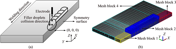
Fig. 1 Schematic picture of GMAW (a) and gridded model (b)

2.3 Tracking solid-liquid interface

Since only one fluid is considered in the simulation, the linear enthalpy-temperature relationship, Eq. (8), is used to track solid–liquid interface and thus the enthalpy of each cell, h, is determined by the fluid temperature, T.

           (8)

where T_s is the solidus temperature and T_l is the liquidus temperature [13, 14].

2.4 Modelling of mushy zone

If the cell temperature is between solidus and liquidus, it means that this cell is in the mushy zone. In this region, the amount of solid phase in the fluid is determined using the temperature ratio. Then, based on critical solid fraction, F_s, and coherent solid fraction, F_Cr, the mushy zone is divided into three parts. Finally, the drag coefficient and fluid viscosity are calculated in each part of the mushy zone as mentioned below.

The first part of the mushy zone is the cells in which the solid fraction is less than coherent solid fraction. In this part, fluid viscosity is calculated according to Eq. (9).

                          (9)

where μ₀ is the dynamic viscosity. The second part of the mushy zone is the cells in which the solid fraction is between coherent solid fraction and critical solid fraction. In this part, the mushy zone is assumed to be a porous media. The fluid viscosity is expressed using Eq. (9) and the drag coefficient is given by Eq. (10).

                         (10)

where C₀ is the constant drag coefficient and δ is the positive zero to avoid dividing zero. Equation (10) represents the frictional dissipation in the mushy zone based on Carman–Koseny equation, which is obtained from Darcy model. In the third part, local solid fraction is greater than the critical solid fraction. According to Eq. (10), there is an infinite resistance against fluid flow and thus fluid flow is stopped [13, 14].

2.5 Boundary conditions

On the top surface according to Eq. (11), arc power, approximated by a Gaussian distribution, transfers to workpiece and dissipates by conduction, convection and radiation [13, 21]. In addition, balance of shear stresses taking into account surface tension shear stress on this surface is described using Eq. (12) [13, 14]. Equation (13) shows the relationship between surface tension and temperature in commercially pure aluminum [22].

       (11)

                           (12)

                   (13)

where n is the direction perpendicular to the free surface, f is the power distribution factor, η is the arc efficiency, I is the welding current, V is the welding voltage, σ_q is the arc flux distribution parameter, x is the longitudinal axis, y is the transverse axis, h_c is the heat transfer coefficient, σ is the Stefan–Boltzmann constant, ε is the radiation emissivity, v_T is the tangential velocity vector, is the temperature coefficient of surface tension, τ is the tangential vector to the free surface and γ is the surface tension [13, 14, 21, 22].

For symmetry boundary, fluid velocity components (u, v and w) and temperature changes according to Eqs. (14) and (15) equal zero [13, 20].

                            (14)

                                    (15)

On the other boundary, heat dissipated by convection and radiation according to Eq. (16) and velocity components are equal to zero according to Eq. (17) [13, 21]. All material properties and parameters that need for the simulations are listed in Table 1. It should be noted that arc efficiency based on LU and KOU [23] measurements is determined.

              (16)

u=υ=w=0                                   (17)

2.6 Initial droplet conditions

The droplets are assumed to be spherical [11]. Based on the experimental measurements, which have been done by FERRARESI et al [25], initial droplet diameter is determined. Initial droplet velocity along negative Z direction is considered equal to electrode feed rate and initial droplet temperature is obtained from the separate simulation results. Droplet generation frequency according to the initial diameter of the droplet and the electrode feed rate is determined by considering the conservation of mass [14]. Initial droplet parameters for different samples are presented in Table 2.

Table 1 Physical properties used in calculations [14, 22–24]

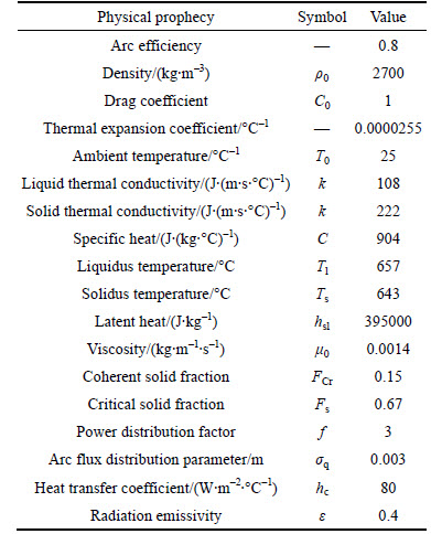
Table 2 Initial droplet conditions used for all samples [11, 25]

2.7 Numerical procedure

In order to simulate GMAW process, the above region of the sample (Fig. 1) is added to the workpiece and is defined as void. To track interface between molten aluminum and void region over time, the simulations in free surface condition are done. As mentioned previously, a source term in the governing equations is used to add mass, momentum and energy of the droplets to the weld pool. The molten droplets form in the void region and then they are accelerated toward the workpiece. After development of the model, all conservation equations are solved by FLOW-3D software through the following steps:

1) Approximation of new speed velocity based on previous time step.

2) Determination of pressure formulation by using generalized minimal residual (GMRES) method and then solution of the energy equation.

3) Update free surface by using VOF method.

The above steps are repeated at each time interval. The convergence criteria for all the equation and minimum time step size during simulation are 0.001 and 0.00005 s, respectively.

3 Experimental procedure

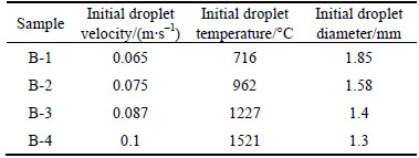
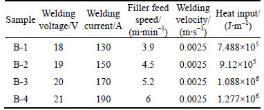
Commercially pure aluminum sheets with a thickness of 5 mm, and 4043 aluminum filler wire with a diameter of 1.2 mm were used to prepare the samples. The chemical compositions of the workpiece and filler wire electrode are given in Table 3. The composition was determined using optical emission spectroscopy. Workpieces with a width of 10 cm were machined out of the sheet and welding experiments were conducted to confirm the calculations under conditions that are listed in Table 4. In all samples, welding speed was 2.5 mm/s and flow rate of shielding gas was 12 L/min. High purity (99.9%) argon was utilized as welding gas. GMA welds were performed on the samples using a direct constant current welding power supply, GAAM Pars Model MIG SP501W, with electrode negative polarity. Before welding, a wire brush was used to remove the oxide layer on the samples. After welding, the welded samples were cut out from middle and then weld bead was etched by using the Poullton’s reagent [26].

Table 3 Chemical composition of commercially pure aluminum and 4043 aluminum filler wire (mass fraction, %)

Table 4 Welding parameters and heat input for all samples

4 Results and discussion

4.1 Weld pool dimensions

Figure 2 shows the comparison of the calculated and experimental results for the samples with the different welding current. The computed weld pool geometry and dimensions agree well with the experimental results. The red region has a temperature above 643 °C and presents the weld pool. Good agreement between the experimental and simulated results confirms the validity of the model. Besides weld pool dimensions, Fig. 2 exhibits the fluid flow pattern using velocity vectors in the weld pool. Due to impinging of droplets during welding, fluid flow pattern alternatively changes in this process. The droplet mass, momentum and energy are transferred to the weld pool by droplet impingement. After disappearance of impingement droplet effects, fluid flow pattern becomes identical in all samples (Fig. 2). The velocity field is generally composed of the counterclockwise vortex (in the right view) that is downward along the weld pool axis and then upward along the pool boundary. The droplet impinging force causes molten metal to flow in a counterclockwise vortex and influences the weld pool depth while the driving forces of surface tension and buoyancy creates a clockwise vortex and influences the weld pool width. Hence, probably droplet impinging force is the dominant driving force in the weld pool and determines fluid flow pattern in the weld pool.

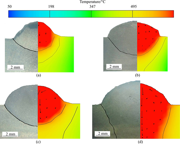
Fig. 2 Comparison of simulation and experimental result for B-1 (a), B-2 (b), B-3 (c) and B-4 (d) samples with different welding current

Figure 3 displays the predicted values of weld pool width and penetration depth for various welding current. In general, the weld pool dimensions increase with increasing the welding current. The increase in the amount of the heat input is the main reason for this behavior. The heat input in arc welding processes is determined by Eq. (18).

                                 (18)

In this equation, H is the heat input and U_Scan is the welding speed [1]. Heat inputs for the different samples according to Eq. (18) are calculated and presented in Table 4. The voltage changes are very small and the welding speed is constant. Thus, the welding current is main parameter that determines the heat input and different values of H has been obtained by changing the welding current. With increasing the welding current and the heat input, both the weld pool width and depth increase (Fig. 3(a)). Except for the sample B-4, the half width of weld pool for all other samples is higher than the weld pool depth and a wide and shallow weld pool has been produced in the samples B-1, B-2 and B-3. As a result, in the welding currents of above 170 A, another parameter affects the weld pool geometry in addition to the heat input.

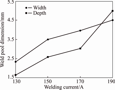
Fig. 3 Simulation weld pool dimension for half width and Penetration depth of weld pool

4.2 Temperature and velocity fields

Figure 4 shows the top view of temperature distribution for the different samples in middle of welding time (t=7.5 s). With increasing the welding current from 130 to 190 A, the temperature distribution lines become wider and the average sample temperature increases too. In order to better evaluate the process, peak temperature in the weld pool for all samples is predicted and shown in Fig. 5. The peak temperature in the weld pool increases with increasing welding current. The increase in the heat input due to increasing the welding current is the reason for the higher average sample temperature and the higher peak temperature in the weld pool.

Figure 6 shows the maximum velocity components in the weld pool during welding against the welding current. All velocity components increase by increasing the welding current. This result supported the results shown in Fig. 2. The main driving force for fluid flow on the surface of the weld pool is the surface tension (Marangoni effect). With increasing the welding current and heat input, the peak temperature, the weld pool dimensions and the temperature difference on the surface of weld pool increase. Hence, fluid flow owing to the buoyancy and surface tension forces increases. The maximum velocity along the X-axis is higher than that along Y-axis, which is attributed to the bigger weld pool along the X-axis than Y-axis.

The main driving force for fluid flow along the Z-axis is resulted from the droplet impinging. Due to the increase in the welding current and filler feed speed, initial droplet velocity and droplet number in a same time increase. As a result, with increasing the welding current, the maximum velocity along the Z-axis increases more compared with the other directions. Because droplets impinge along the Z-axis and the maximum velocity along the Z-axis is created, the main driving force in the weld pool during GMAW is the impinging of droplets.

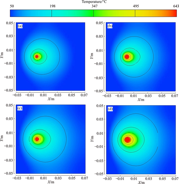
Fig. 4 Top view simulation of temperature distribution for B-1 (a), B-2 (b), B-3 (c) and B-4 (d) samples in middle of welding time (t=7.5 s)

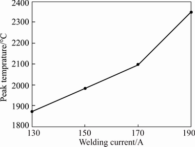
Fig. 5 Maximum weld pool temperature with welding current process

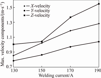
Fig. 6 Maximum velocity component in weld pool during process against welding current

Therefore, the driving forces of buoyancy, surface tension and droplet impinging can affect the convective heat transfer and the weld pool dimensions. Further, the increase in weld pool penetration depth (Fig. 3(a)) and the higher velocity along the z-axis (Fig. 6) indicate the more important role of the droplet impinging force in the welding current of 190 A.

The heat-affected zone (HAZ) in commercial purity aluminum is a region whose maximum temperature ranges from 377 °C (a temperature high enough to alter the base material’s structure) to 643 °C (solidus temperature). In this zone, although the base metal is not melted, the structure and grain size change due to the welding heat input [27].Figure 7 exhibits temperature distribution in the cross section of the samples B-1, B-2, B-3, and B-4. In Fig. 7, the red region has a temperature above 643 °C (weld pool) and blue region has a temperature under 377 °C. In Fig. 7(a), the width of the HAZ on the top surface of the cross section has been specified. Figure 8 reveals the changes in the width of the HAZ with the welding current. The width of the HAZ increases with increasing the welding current. As previously mentioned, the increase in the welding current causes to an increase in the heat input, which is the reason of the larger width of the HAZ.

4.3 Dimensionless numbers

Dimensionless Peclet, Grashof and surface tension Reynolds numbers by using Eqs. (19)–(21) are calculated, respectively.

                             (19)

                            (20)

                        (21)

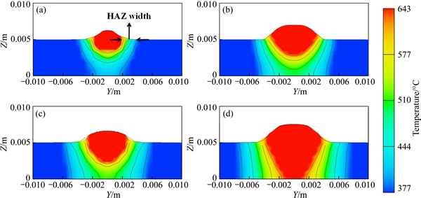
Fig. 7 HAZ temperature distribution in cross section in middle of process for B-1 (a), B-2 (b), B-3 (c) and B-4 (d)

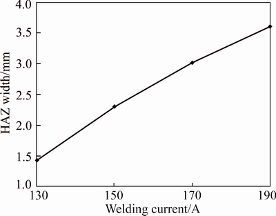
Fig. 8 HAZ width changes with welding current

where U_R is the average weld pool velocity, L_R is the weld pool half width, L_B is the characteristic length of buoyancy force (approximately one-eighth the weld pool width), and ΔT is the difference between the maximum and solidus temperatures [21, 28].

Figure 9 shows Peclet number variations as a function of the welding current. Peclet number is used for assessment of the relative importance of convective and conductive heat transfer in the weld pool [28]. Because Peclet number is greater than 1, convective heat transfer is dominant in the weld pool for all welding current. Furthermore, with increasing the welding current, because of stronger driving forces and bigger weld pool, Peclet number increases and hence convective heat transfer in the weld pool becomes stronger.

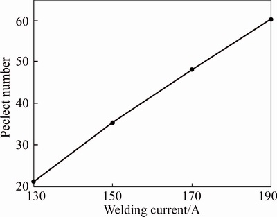
Fig. 9 Peclet number variations over welding current

Figure 10 shows changes in Grashof number with increasing the welding current. Grashof number is directly related to the buoyancy force [28]. As exhibited in Fig. 10, due to the higher maximum temperature and temperature gradient in the weld pool and hence the higher density change in the weld pool, Grashof number and the buoyancy force increase with increasing the welding current.

Plot of surface tension Reynolds number versus the welding current is shown in Fig. 11. Surface tension Reynolds number is an index of the surface tension force [28]. As revealed in Fig. 11, the increase in the welding current causes to the increase in the surface tension Reynolds number and surface tension force. This is because of the increase in peak temperature and more temperature gradient in the weld pool and hence the higher surface energy change.

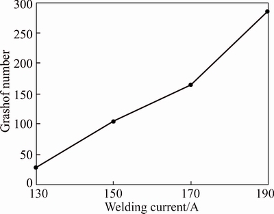
Fig. 10 Grashof number changes versus welding current

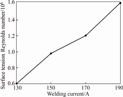
Fig. 11 Surface tension Reynolds number against welding current

Dimensionless numbers ratios represent contribution rate of driving forces in the weld pool. Because surface tension Reynolds number is much more than Grashof number, surface tension force compared to buoyancy force have much greater contribution to the weld pool fluid flow. In addition, as previously mentioned, the droplet impinging is the main driving force in the weld pool. Thus, the droplet impinging force, surface tension force and buoyance force have much greater contribution in weld pool fluid flow, respectively.

5 Conclusions

In this research, the influences of welding current on the weld pool geometry during gas metal arc welding of commercial purity aluminium are predicted through three dimensional modelling of heat transfer and fluid flow. The main results of this study are:

1) The geometry of fusion zone predicted from the three dimensional transient heat transfer and fluid flow model using FLOW-3D software is in good agreement with the corresponding experimental results. Hence, estimation of the size and shape of the GMA welds is possible by using the model presented here and there is no longer need to carry out experiments.

2) With increasing the welding current, average sample temperature, peak temperature and velocity components in the weld pool, width of the HAZ, and weld pool dimensions increase due to the higher heat input and droplet impinging force.

3) The increase in the welding current from 130 to 190 A increases Peclet, Grashof and surface tension Reynolds numbers significantly. It means that contribution of convective heat transfer compared to conductive heat transfer increases extremely, resulting from the increase in the weld pool size and velocity due to the stronger buoyancy force, surface tension force, and droplet impinging force.

4) The main driving forces that affected fluid flow in the weld pool are droplet impinging force, surface tension force and buoyancy force, respectively.

References

[1] WEMAN K, LINDEN G. MIG welding guide [M]. Cambridge: Woodhead Publishing Limited, Abington Hall, 2006.

[2] PERRET W, SCHWENK C, RETHMEIER M. Comparison of analytical and numerical welding temperature field calculation [J]. Computational Materials Science, 2010, 47: 1005–1015.

[3] YANG Z, DEBROY T. Modeling macro-and microstructures of gas- metal-arc welded HSLA-100 steel [J]. Metallurgical and Materials Transactions B, 1999, 30B: 483–493.

[4] FARZADI A, SERAJZADEH S, KOKABI A H. Modelling of transport phenomena in gas tungsten arc welding [J]. Archives of Materials Science and Engineering, 2007, 28(7): 417–420.

[5] CHO M H, FARSON D F. Understanding bead hump formation in gas metal arc welding using a numerical simulation [J]. Metallurgical and Materials Transactions B, 2007, 38B: 305–319.

[6] KUMAR, DEBROY T. Guaranteed fillet weld geometry from heat transfer model and multivariable optimization [J]. International Journal of Heat and Mass Transfer, 2004, 47: 5793–5806.

[7] KIM C H, ZHANG W, DEBROY T. Modeling of temperature field and solidified surface profile during gas metal arc fillet welding [J]. Journal of Applied Physics, 2003, 94(4): 2667–2679.

[8] XU Guo-xiang, WU Chuan-song. Numerical analysis of weld pool geometry in globular-transfer gas metal arc welding [J]. Frontiers of Materials Science in China, 2007, 1(1): 24–29.

[9] AZAR AMIN S, SIGMUND K, AKSELSEN M. Determination of welding heat source parameters from actual bead shape [J]. Computational Materials Science, 2012, 54: 176–182.

[10] KIM I S, BASU A. A mathematical model of heat transfer and fluid flow in the gas metal arc welding process [J]. Journal of Materials Processing Technology, 1998, 77: 17–24.

[11] WANG Y, TSAI H L. Impingement of filler droplets and weld pool dynamics during gas metal arc welding process [J]. International Journal of Heat and Mass Transfer, 2001, 44: 2067–2080.

[12] ARGHODE V K, KUMAR A, SUNDARRAJ S, DUTTA P. Computational modeling of GMAW process for joining dissimilar aluminum alloys [J]. An International Journal of Computation and Methodology, 2008, 53(4): 432–455.

[13] CAO Z, YANG Z, CHEN X L. Three-dimensional simulation of transient GMA weld pool with free surface [J]. Welding Journal, 2004, 83: 169–176.

[14] CHO M H, LIM Y C, FARSON D F. Simulation of weld pool dynamics in the stationary pulsed gas metal arc welding process and final weld shape [J]. Welding Journal, 2006, 85: 271–283.

[15] LIM Y C, FARSON D F, CHO M H, CHO J H. Stationary GMAW-P weld metal deposit spreading [J]. Science and Technology of Welding and Joining, 2009, 14(7): 625–635.

[16] HU J, GUO H, TSAI H L. Weld pool dynamics and the formation of ripples in 3D gas metal arc welding [J]. International Journal of Heat and Mass Transfer, 2008, 51: 2537–2552.

[17] GUO H, HUB J, TSAI H L. Formation of weld crater in GMAW of aluminum alloys [J]. International Journal of Heat and Mass Transfer, 2009, 52: 5533–5546.

[18] RAO Z H, ZHOU J, LIAO S M, TSAI H L. Three-dimensional modeling of transport phenomena and their effect on the formation of ripples in gas metal arc welding [J]. Journal of Applied Physics, 2010, 107: 1–14.

[19] CHEN J, SCHWENK C, WU C S, RETHMEIER M. Predicting the influence of groove angle on heat transfer and fluid flow for new gas metal arc welding processes [J]. International Journal of Heat and Mass Transfer, 2012, 55: 102–111.

[20] LU F, WANG H P, MURPHY A, CARLSON B E. Analysis of energy flow in gas metal arc welding processes through self-consistent three-dimensional process simulation [J]. International Journal of Heat and Mass Transfer, 2014, 68: 215–223.

[21] FARZADI A, SERAJZADEH S, KOKABI A H. Modeling of heat transfer and fluid flow during gas tungsten arc welding of commercial pure aluminum [J]. The International Journal of Advanced Manufacturing Technology, 2008, 33: 258–267.

[22] GUO H, HU J, TSAI H L. Three-dimensional modeling of gas metal arc welding of aluminum alloys [J]. Journal of Manufacturing Science and Engineering, 2010, 132: 021011.

[23] LU M J, KOU S. Power inputs in gas metal arc welding of aluminum-Part 1 [J]. Welding Journal, 1989, 38: 382–388.

[24] FARZADI A, SERAJZADEH S, KOKABI A H. Investigation of weld pool in aluminum alloys: Geometry and solidification microstructure [J]. International Journal of Thermal Sciences, 2010, 49: 809–819.

[25] FERRARESI V A, FIGUEIREDO K M, HIAP ONG T. Metal transfer in the aluminum gas metal arc welding [J]. Brazilian Society of Mechanical Sciences and Engineering, 2003, 25(3): 229–234.

[26] Metallography and microstructures [M]. Ohio: ASM International, 1992.

[27] BAY B, HANSEN N. Recrystallization in commercially pure aluminum [J]. Metallurgical Transactions A, 1984, 15(2): 287–297.

[28] HE Y, FUERSCHBACH P W, DEBROY T. Heat transfer and fluid flow during laser spot welding of 304 stainless steel [J]. Journal of Physics D: Applied Physics, 2003, 36: 1388–1398.

(Edited by HE Yun-bin)

Cite this article as: Farzadi A, Morakabiyan Esfahani M, Alavi Zaree S R. Theoretical and experimental investigation of gas metal arc weld pool in commercially pure aluminum: Effect of welding current on geometry [J]. Journal of Central South University, 2017, 24(11): 2556–2564. DOI:https://doi.org/10.1007/s11771-017-3669-4.

Received date: 2016-07-01; Accepted date: 2017-08-15

Corresponding author: Farzadi A, PhD; Tel: +98–21–64545581; E-mail: farzadi@aut.ac.ir