J. Cent. South Univ. (2017) 24: 2596-2604

DOI: https://doi.org/10.1007/s11771-017-3673-8

Stochastic noise identification in a stray current sensor

XU Shao-yi(许少毅)¹, XING Fang-fang(邢方方)², LI Wei(李威)¹, WANG Yu-qiao(王禹桥)¹

1. School of Mechanical and Electrical Engineering, China University of Mining and Technology,Xuzhou 221116, China;

2. School of Mechatronic Engineering, Xuzhou College of Industrial Technology, Xuzhou 221116, China

Central South University Press and Springer-Verlag GmbH Germany, part of Springer Nature 2017

Abstract: The Allan variance analysis method is used to identify the stochastic noise in the stray current sensor. The stray current characteristic is firstly introduced. Then the optical configuration and the signal processing method of the stray current sensor are illustrated. Moreover, the cause of the stochastic noise in the stray current sensor is analyzed. The calculation method of the stochastic noise coefficient is presented in detail. And the feasibility of the stochastic noise identification with the Allan variance analysis method is evaluated. Furthermore, the zero-drift signal acquisition experiment is conducted to identify the stochastic noise in the stray current sensor. According to the experimental result, the bias instability noise, the quantization noise and the white noise are identified as the major stochastic noise. Finally, the experiment on the direct-current signal acquisitions is conducted, whose results indicate that the signal drift of the measured direct-current is mainly caused by the major stochastic noise. And the suppression methods of the major stochastic noise are proposed.

Key words: stochastic noise; stray current; optical fiber current sensor

1 Introduction

Optical fiber current sensor (OFCS) has drawn wide attention in the past three decades. According to the signal detection methods, OFCS is usually divided into two types: interferometer [1, 2] and polarimetric [3–6]. Previous work has focused on eliminating the effect of various errors in OFCS, including the linear birefringence error of sensing fiber, the phase retardation error of imperfect quarter wave-plate, the alignment error of fused optical fibers, and the modulation error of polarization controller. Among them, the elimination methods for linear birefringence error have been improved. This has been achieved by adding large amounts of circular birefringence to the sensing fiber  [7, 8], utilizing a fiber polarization rotator [9], and using an annealed sensing coil [10]. Moreover, ways to suppress the effect of imperfect wave-plate have been proposed, which include an inherent temperature compensation scheme [10] or an electronic peak divide signal processing scheme [11]. Furthermore, an elimination method on alignment error has been presented based on the modulation angle of polarization controller [12]. Based on these results, the performance of the OFCS has been greatly improved, including its sensitivity and precision. And OFCS has been applied in the electrowinning industry [13] and the electric power transmission [14]. Furthermore, we will use the OFCS to measure the stray current in the urban mass transit system, which will be called stray current sensor in this work.

In the urban mass transit system, the measurement accuracy of the stray current is not greater than 0.4%. It means that the measurement error induced by the stochastic noise should be decreased in stray current sensor. However, little attention has been paid to the effect of the stochastic noise. Thus, the question “how to identify the stochastic noise?” should be solved. It is noted that Allan variance analysis method is a time-based domain analysis approach originally developed to study the frequency stability of precision oscillators. Application of this method has been widely extended to other areas, such as the noise identification of inertial sensor [15] or optical tweezer [16]. It can be applied to determine the characteristic of the underlying stochastic processes that give rise to the data noise. Therefore, the Allan variance analysis method may be suited for identifying the stochastic noise in stray current sensor.

In this work, we introduce the stray current characteristic firstly. The optical configuration and the signal processing method of stray current sensor are illustrated. Then the identification principle of stochastic noise is proposed based on the Allan variance analysis method. The cause of the typical stochastic noise is analyzed. The calculation method of the stochastic noise coefficient is presented. And the feasibility of the stochastic noise identification with the Allan variance analysis method is evaluated. Moreover, two experiments are conducted to identify the stochastic noise and then evaluate the effect of the stochastic noise. The experiment setup is described in detail. The first experiment is conducted to collect the zero-drift signal of stray current sensor, which is used to identify the stochastic noise. The second experiment is the direct-current signal acquisition from 0.5 A to 2.5 A, which is used to evaluate the effect of the stochastic noise.

2 Stray current characteristic

The urban mass transit system usually adopts the direct-current traction power supply system [17]. The traction current of the train is powered by the substation through the overhead line. And the running rail is used as the return conductor of the traction current. This arrangement mainly focuses on economic considerations since it does not require the installation of an additional return conductor [18]. However, the resistance of the running rail to ground is not infinite. And a portion of the traction current will leak into the ground, which is known as the stray current. Once the stray current flows in the buried pipeline (such as the gas pipeline, the oil pipeline and the water pipeline), the electrochemical corrosion might occur in the outflow region. There has been evidence that the corrosion can shorten the life cycle, strength and durability of the buried pipeline [19]. In a few extreme cases, some severe accidents (such as a serious gas explosion) have occurred as a result of stray current corrosion. The stray current generation process is shown in Fig. 1.

Fig. 1 Stray current generation process: TPS–traction substation

According to the China standard CJJ 49–1992 and the European standard EN 50122–2, the stray current corrosion status can be evaluated based on the stray current measurement. We have conducted the field test to study the stray current characteristic. And the test results have been shown in Fig. 2. We can find that the magnitude of the stray current is about in the range between –53.9 A and 42.5 A. And its frequency is not greater than 10.94 Hz, which is in consistence with the results of Ref. [20]. It is noted that the Hall sensor has been applied in our field test. It is an active sensor, which requires a constant current source. It is known that the passive sensor should be most appropriate in the corrosion condition. Moreover, we found that the Hall sensor is easy to be interfered by the external electromagnetic field in our field test. Thus, considering that the OFCS has the advantages of passive sensing and anti-electromagnetic interference, it might be one of the best choices to measure the stray current.

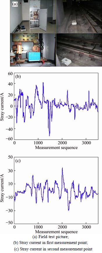
Fig. 2 Field test results on stray current:

3 Sensor configuration

The optical configuration of the stray current sensor is shown in Fig. 3, which includes a broadband source, a polarizer, a coupler, a sensing head, a mirror, a polarization controller (PC), a polarization beam splitter (PBS), a high-speed optical power meter (OPM) and a computer. The sensing head is mainly composed of a multilayer solenoid and the sensing fiber. A heat insulation cavity is set between the solenoid and sensing fiber, which fills the glass cotton to cut off the heat- transfer path. The stray current in the buried pipeline enters into the solenoid by the connector and then induce an axial magnetic field in the solenoid. Moreover, the non-uniform part of the axial magnetic field in the solenoid is isolated by the metal casings made of Ferro- manganese.

Fig. 3 Optical configuration of stray current sensor:

In the stray current sensor, the light beam from the broadband source firstly passes through the polarizer to form a linearly polarized light. The linearly polarized light is then coupled into the sensing fiber, where the Faraday effect occurs due to the axial magnetic field. The plane of polarization is rotated through the Faraday angle in the sensing fiber. The mirror attached at the end of the sensing fiber reflects the polarized light. When the reflected light propagates back to the sensing fiber, the second Faraday effect occurs in the same magnetic field. Moreover, the PC is used to modulate the plane of polarization through 45°. The modulation light travels into the PBS, which splits into the orthogonally optical signals. They are detected immediately by the optical power meter. Finally, the detection results of the power meter are sent to the computer by RS232 interface.

In this work, we define the parameters a and b as the inside and outer radius of multilayer solenoid, which are 0.032 m and 0.054 m, respectively. The parameters L and l are defined as the lengths of multilayer solenoid and uniform magnetic field, which are about 0.39 m and 0.17 m, respectively. The stray current sensor applies the polarization division multiplexing (PDM) detection to process its output signals [4], which is shown by Eq. (1). It is noted that the static power signals P_sx and P_sy are detected when the stray current is zero in the solenoid, which is usually carried out at 3:00 AM every day. Moreover, the dynamic power signals P_dx and P_dy are detected when the stray current is not zero in the solenoid.

                               (1)

where I is the stray current in the solenoid, A; V is the Verdet constant of sensing fiber, μrad/A; n is the number of turns of sensing fiber; n₁ and n₂ are the numbers of turns of multilayer solenoid along the horizontal and vertical direction, which are 639.7 /m and 545.2 /m, respectively. The s represents the sensitivity of stray current sensor.

4 Identification principle of stochastic noise in stray current sensor

The signal of the stray current sensor is collected with sampling time τ₀, which is defined as I=[I₁, I₂, …, I_z]^T. The collection signal is divided into M groups. Each group contains n successive data points, which is defined as one cluster (n≤z/2). Associated with each cluster, a time τ, is equal to nτ₀. The Allan variance σ²(τ) of the collection signal can be calculated as follows [21, 22]:

         (2)

where M=, (is the floor function); is the average value of the kth cluster, A.

Five typical stochastic noises are considered in stray current sensor, which are white noise, quantization noise, bias instability noise, brown noise and ramp noise respectively. The white noise reflects the ultimate precision of the stray current sensor, which is mainly caused by the thermal noise and the shot noise at the photoelectric detector of the power meter. The quantization noise determines the minimum resolution of the stray current sensor, which is mainly caused in the conversion from the Faraday rotation signal to the digital quantity by the power meter. The bias instability noise is mainly caused by the output power instability of the broadband source. The brown noise may be caused by the index correlated noise with the long correlation time in stray current sensor. The comprehensive relationship between Allan variance and the power spectral density (PSD, for short) function of the stochastic noise can be given by the following equation [23]:

               (3)

where S(f) is the PSD function of the stochastic noise and f is the frequency.

It is known that the white noise is the stochastic noise with a constant PSD. Thus, the PSD function of white noise can be defined as N². Moreover, the PSD function of quantization noise can be defined as (2πfQ)²τ; the PSD function of bias instability noise can be defined as B²/2πf; the PSD function of brown noise can be defined as [W/(2πf)]². Among them, N is defined as the white noise coefficient, Q is defined as the quantization noise coefficient, A·s; B is defined as the bias instability noise coefficient, A; And W is defined as the brown noise coefficient, Thus, the Allan standard deviations of the first four stochastic noises in stray current sensor can be derived based on Eq. (3), which is shown as follows [24, 25]:

                    (4)

Last but not least, the ramp noise is related to the long term stability of photoelectric elements and working condition of stray current sensor. One main source of this noise is the slowly-varying temperature, which lasts for a long time. Its Allan standard deviation can be obtained based on Eq. (2), which is shown as Eq. (5). It is noted that R is defined as the ramp noise coefficient, A/s.

                            (5)

It is assumed that these stochastic noises in stray current sensor are independent of each other [25, 26]. According to Eqs. (4) and (5), the total Allan standard deviation can be expressed as

                 (6)

where x₁=N, x₂=Q, x₃=B, x₄=W, x₅=R.

Equation (6) can also be expressed in matrix form σ=A·X as follows:

                             (7)

where the parameter m is the maximum value of data points in each cluster.

Thus, the least-square method is applied to solve the noise coefficients from x₁ to x₅ in Eq. (7). Its objective function is given as

                  (8)

where the fitting Allan standard deviation is defined as σ_e, which is equal to A·X_e. And the vector X_e is the fitting results of noise coefficients. According to Eq. (8), the expression for the Allan standard deviation is obtained as a function of the cluster time τ. And a log-log plot of σ(τ) versus τ can be drawn in the stochastic noise identification.

The simulations have been conducted to evaluate the feasibility of the stochastic noise identification with the Allan variance analysis method. In these simulations, the noise sequences (CN) are both composed of the white noise (WN), the bias instability noise (BIN), the brown noise (BN) and the ramp noise (RN). The RN sequence is simulated as And the coefficient R is set as 1.0×10^–5. For the first simulation, the WN is set as the first major noise and the BIN is set as the second major noise. The actual value of these independent noise coefficients can be calculated based on their corresponding PSD function. Moreover, the Allan standard variance (ASD) of the composed noise can be calculated based on Eq. (2) and its fitting results can be calculated based on Eq. (8). Thus, the actual value and identification value are shown in Table 1. The noise sequences and the ASD curve are shown in Fig. 4. It can be found that the WN and BIN are identified as the first and second major noise respectively, which is consistent with the actual results.

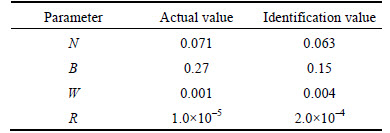
Table 1 Actual value and identification value for first simulation noise sequence

For the second simulation, the BIN is set as the first major noise and the WN is set as the second major noise. Similarly, the actual value and identification value are shown in Table 2. The noise sequences and the ASD curve are shown in Fig. 5. According to Table 2 and Fig. 5, we can find that the identification results are correct, which indicates that the Allan variance analysis method can be applied to the identification of the stochastic noise in the stray current sensor.

5 Experimental results and discussion

The experiments are conducted based on the configuration shown in Fig. 3. In our experiments, the broadband source is an amplified spontaneous emission (ASE) source (B&A Technology Co. Ltd., model AS 4513). Its operation wavelength is in the range from 1525 nm to 1565 nm. Its spectrum flatness is not larger than 1.5 dB. And its output power is about 11.9 dB·m. The high-speed optical power meter is produced by EXFO Co. Ltd., whose mode is PM-1623. The sensing fiber is the low birefringence fiber (Oxford Electronics Co. Ltd., model LB 1550-125), whose linear birefringence is about 4°/4m at 20 °C. Moreover, the extinction ratio of the polarizer is about 35 dB tested by the extinction ratio meter (FiberPro Co. Ltd., model ER2200). In the computer, the data acquisition system is designed to obtain the detection results of the power meter based on Labview software. And the actual and fitting Allan variance results are both calculated using MATLAB software based on the acquired data.

Our experiments include two parts: one is the zero-drift signal acquisition without stray current, which is used to identify the stochastic noise in the stray current sensor based on Allan variance analysis method; the other is the direct-current signal acquisition, which is used to evaluate the effect of the stochastic noise.

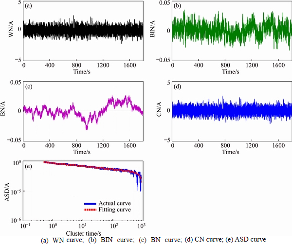
Fig. 4 First simulation noise sequence and its Allan variance curve:

Table 2 Actual value and identification value for second simulation noise sequence

5.1 Stochastic noise identification based on zero-drift signal acquisition

In this experiment, the number of turns of the sensing head is 2 in the stray current sensor. The experimental conditions are described as follows: 1) The stray current is zero; 2) The stray current sensor is installed on a vibration isolation platform; 3) The experiment is conducted at 20 °C; 4) The sampling frequency of the power meter is defined as F_s, which is about 2 Hz. In this experiment, the static power signals P_sy and P_sx are about 2.2546 mW and 3.2666 mW, respectively. The dynamic power signals P_dy and P_dx have been collected for half an hour, which are shown in Figs. 6(a) and (b). And the sensor output can be calculated based on Eq. (1), which is shown in Fig. 6(c). It is noted that the sensitivity is about 0.0136 A^–1. Thus, the zero drift signal of the stray current sensor can be calculated, which is shown in Fig. 7(a). We can find that the zero-drift signal is random within a range of –0.008 A to 0.0688 A. Moreover, the Allan variance of the zero-drift signal can be calculated based on Eq. (2), which is shown as the solid blue curve in Fig. 7(b). And the fitting Allan variance can be calculated based on Eq. (8), which is shown as the dotted red curve in Fig. 7(b).

According to the fitting results, the white noise coefficient N is equal to 1.461×10^–4 the quantization noise coefficient Q is equal to 6.67×10^–4A·s; the bias instability noise coefficient B is equal to 7.504×10^–4 A; the brown noise coefficient W is equal to 1.685×10^–5 and the ramp coefficient R is equal to 2.977×10^–5 A/s. We can find that the major stochastic noises are the bias instability noise, the quantization noise and the white noise.

5.2 Direct-current signal acquisitions to evaluate effect of stochastic noise

According to the field test results in Section 2, the stray current belongs to the low-frequency current. Thus, we substitute the direct-current for the stray current under laboratory conditions. The results of the direct-current signal acquisitions are shown in Fig. 8. The sampling frequency F_s of the power meter is also about 2 Hz. The static power signals P_sy and P_sx are about 2.2529 mW and 3.2607 mW, respectively. Each current signal acquisition lasts for 90 s. And the acquisitions from 0.5 A to 2.0 A are conducted twice, whose detailed results are shown in Fig. 9.

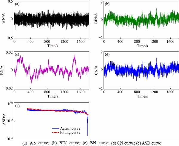
Fig. 5 Second simulation noise sequence and its Allan variance curve:

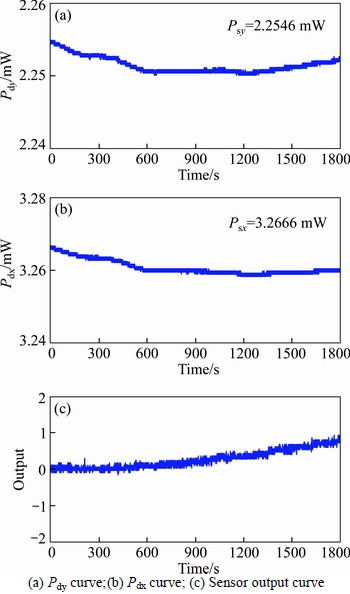
Fig. 6 Dynamic power signals and sensor output:

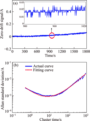
Fig. 7 Zero-drift signal (a) and its Allan variance curve (b) of stray current sensor

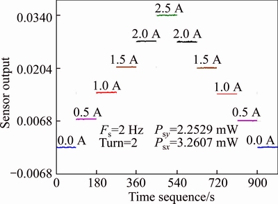
Fig. 8 Results of direct-current signal acquisitions

According to Figs. 9(a) and (b), the measured current signal is within a range of 0.498 A to 0.539 A. Compared with the expected value 0.50 A, the drift value is within a range of –0.002 A to 0.039 A. Then, according to Fig. 9(c) and (d), the measured current signal is within a range of 1.003 A to 1.044 A. Compared with the expected value 1.00 A, the drift value is within a range of 0.003 A to 0.044 A. Moreover, according to Figs. 9(e) and (f), the measured current signal is within a range of 1.487 A to 1.523 A. Compared with the expected value 1.50 A, the drift value is within a range of –0.013 A to 0.023 A. Finally, according to Figs. 9(g) and (h), the measured current signal is within a range of 1.990 A to 2.011 A. Compared with the expected value 2.00 A, the drift value is within a range of –0.01 A to 0.011 A. Thus, we believe that the signal drift of the measured direct-current is mainly caused by the bias instability noise, the quantization noise and the white noise, which have been proven to cause the zero-drift signal within a range of –0.008 A to 0.0688 A.

According to the above experiment results, the three major stochastic noises really affect the measurement accuracy of the stray current sensor. Since the quantization noise is closely related to the conversion accuracy of the A/D converter of the power meter, one of the methods to suppress the quantization noise is raising the digits of the A/D converter. Moreover, our power meter applies two InGaAs detectors. The thermal noise and the shot noise are both the function of the detection bandwidth of the power meter [27]. The former is also proportional to the operating temperature of the InGaAs detector. And the latter is also proportional to the dark current at the InGaAs detector [28]. Thus, the methods to suppress the white noise include the detection bandwidth compression by optimizing the amplification circuit in the power meter, the low-temperature condition establishment and the dark current reduction for the InGaAs detector. It is known that the active surface of the InGaAs detector is usually 1 mm or 3 mm in diameter, whose dark current is about 2 nA or 25 nA at 5 V. The active surfaces of the InGaAs detectors in our power meter are both 1 mm in diameter. Furthermore, the stray current sensor applies the PDM detection, which is shown in Eq. (1). The PDM detection considers the static power signals. It indicates that broadband source with the high power stability is essential to suppressing the bias instability noise. The total power stability of a broadband source can be expressed as ±half the difference between the maximum and minimum power values measured in the period, which is usually 15 min or 8 h. For example, the total power stability of the specific broadband source (EXFO Co. Ltd., model FLS-2200) is up to ± 0.015 dB in 8 h, which may suppress the bias instability noise better than the used broadband source (B&A Technology Co. Ltd., model AS 4513) in this work.

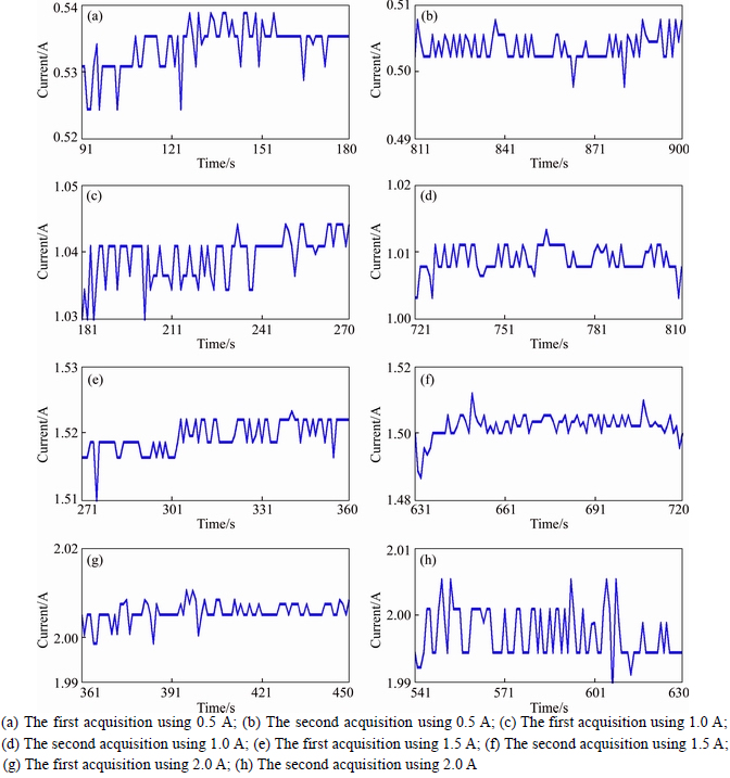
Fig. 9 Detailed results of signal acquisitions from 0.5 A to 2.0 A:

6 Conclusions

In this work, the Allan variance analysis method is used to identify the stochastic noise in the stray current sensor. First, the stray current characteristic is introduced, whose magnitude is about in the range between –53.9 A and 42.5 A. And its frequency is not greater than 10.94 Hz. The optical configuration of stray current sensor is illustrated. And the PDM detection is applied to process the output signal of this sensor. Moreover, the cause of the stochastic noise in stray current sensor is analyzed. The calculation method of the stochastic noise coefficient is presented in detail. And the feasibility of the stochastic noise identification with the Allan variance analysis method is evaluated. Furthermore, the zero-drift signal acquisition experiment is conducted to identify the stochastic noise in stray current sensor. According to the experimental result, the bias instability noise, the quantization noise and the white noise are identified as the major stochastic noise. Finally, the experiment on direct-current signal acquisitions is conducted. And the drift values of the measured direct-current from 0.5 A to 2.0 A are mainly in the range of –0.008 A to 0.0688 A, which is the zero-drift range of stray current sensor. Thus, we believe that the signal drift of the measured direct-current is mainly caused by the major stochastic noise. In addition, the suppression methods of the major stochastic noise are proposed.

References

[1] YU J, ZHANG C X, LI C S, WANG X X, LI Y, FENG X J. Influence of polarization-dependent crosstalk on scale factor in the in-line Sagnac interferometer current sensor [J]. Optical Engineering, 2013, 52(11): 722–730.

[2] OH M C, CHU W S, KIM K J, KIM J W. Polymer waveguide integrated-optic current transducers [J]. Optics Express, 2011, 19(10): 9392–9400.

[3] ZHANG H, QIU Y S, HUANG Z T, JIANG J Z, LI G M, CHEN H X, LI H. Temperature and vibration robustness of reflecting all-fiber current sensor using common single-mode fiber [J]. Journal of Lightwave Technology, 2014, 32(22): 3709–3715.

[4] XU S Y, LI W, XING F F, WANG Y Q. Polarimetric current sensor based on polarization division multiplexing detection [J]. Optics Express, 2014, 22(10): 11985–11994.

[5] HUANG D, SRINIVASAN S, BOWERS J E. Compact Tb doped fiber optic current sensor with high sensitivity [J]. Optics Express, 2015, 23(33): 29993–29999.

[6] ZHANG H Y, DONG Y K, LEESON J, CHEN L, BAO X Y. High sensitivity optical fiber current sensor based on polarization diversity and a Faraday rotation mirror cavity [J]. Applied Optics, 2013, 50(6): 924–929.

[7] XU S Y, LI W, WANG Y Q, XING F F. Stray current sensor with cylindrical twisted fiber [J]. Applied Optics, 2014, 53(24): 5486–5492.

[8] ZHANG C X, LI C S, WANG X X, LI L J, YU J, FENG X J. Design principle for sensing coil of fiber-optic current sensor based on geometric rotation effect [J]. Applied Optics, 2011, 51(18): 3977–3988.

[9] ZHOU S, ZHANG X. Simulation of linear birefringence reduction in fiber-optical current sensor [J]. IEEE Photonics Technology Letters, 2007, 19(17): 1568–1570.

[10] BOHNERT K, GABUS P, NEHRING J, BRANDLE H. Temperature and vibration insensitive fiber-optic current sensor [J]. Journal of Lightwave Technology, 2002, 20(2): 267–276.

[11] SHORT S X, ARRUDA De J U, TSELIKOV A A, BLAKE J N. Elimination of birefringence induced scale factor errors in the in-line Sagnac interferometer current sensor [J]. Journal of Lightwave Technology, 1998, 16(10): 1844–1850.

[12] XU S Y, LI W, WANG Y Q, XING F F. Effect and elimination of alignment error in an optical fiber current sensor [J]. Optics Letters, 2014, 39(16): 4751–4754.

[13] BOHNERT K, BRANDLE H, BRUNZEL M G, GABUS P, GUGGENBACH P. Highly accurate fiber-optic DC current sensor for the electrowinning industry [J]. IEEE Transactions on Industry Applications, 2007, 43(1): 180–187.

[14] SHEN T, FENG Y, SUN B C, WEI X L. Magnetic field sensor using the fiber loop ring-down technique and an etched fiber coated with magnetic fluid [J]. Applied Optics, 2016, 55(4): 673–678.

[15] LI J T, FANG J C. Sliding average Allan variance for inertial sensor stochastic error analysis [J]. IEEE Transactions on Instrumentation and Measurement, 2013, 62(12): 3291–3300.

[16] CZERWINSKI F, RICHARDSON A C, ODDERSHEDE L B. Quantifying noise in optical tweezers by Allan variance [J]. Optics Express, 2009, 17(15): 13255–13269.

[17] XU S Y, LI W, XING F F, WANG Y Q. Novel predictive model for metallic structure corrosion status in presence of stray current in DC mass transit systems [J]. Journal of Central South University, 2014, 21(3): 956–962.

[18] XU S Y, LI W, WANG Y Q. Effects of vehicle running mode on rail potential and stray current in DC mass transit systems [J]. IEEE Transactions on Vehicular Technology, 2013, 62(8): 3569–3580.

[19] XU S Y, LI W. Research on stray current corrosion evaluation of buried metallic pipeline in an urban rail transit system [J]. International Journal of Electrochemical Science, 2015, 10(7): 5950–5960.

[20] DAROWICKI K, ZAKOWSKI K. A new time-frequency detection method of stray current field interference on metal structures [J]. Corrosion Science, 2004, 46(5): 1061–1070.

[21] LV H F, ZHANG L, WANG D J, WU J. An optimization iterative algorithm based on nonnegative constraint with application to Allan variance analysis technique [J]. Advances in Space Research, 2014, 53(5): 836–844.

[22] NIU X J, CHEN Q J, ZHANG Q, ZHANG H P, NIU J M, CHEN K J, SHI C, LIU J N. Using Allan variance to analyze the error characteristics of GNSS positioning [J]. GPS Solutions, 2014, 18(2): 231–242.

[23] LI J T, FANG J C. Not fully overlapping Allan variance and total variance for inertial sensor stochastic error analysis [J]. IEEE Transactions on Instrumentation and Measurement, 2013, 62(10): 2659–2672.

[24] DRAGANOVA K, KMEC F, BLAZEK J, PRASLICKA D, HUDAK J, LASSAK M. Noise analysis of magnetic sensors using Allan variance [J]. Acta Physica Polonica A, 2014, 126(1): 394–395.

[25] EI-SHEIMY N, HOU H Y, NIU X J. Analysis and modeling of inertial sensors using Allan variance [J]. IEEE Transactions on Instrumentation and Measurement, 2008, 57(1): 140–149.

[26] ZHANG Q, WANG L, GAO P Y, LIU Z J. An innovative wavelet threshold denoising method for environmental drift of fiber optic gyro [J]. Mathematical Problems in Engineering, 2016, ID: 9017481.

[27] RABELO R C, CARVALHO De R T, BLAKE J. SNR enhancement of intensity noise-Limited FOGs [J]. Journal of Lightwave Technology, 2000, 18(12): 2146–2150.

[28] TENG F, JIN J, ZHANG Z C, DU S S, SONG N F, ZHANG C X. Noise decomposition and parameter optimization method for high sensitivity fiber optic gyroscope [J]. Science China Technological Sciences, 2015, 58(6): 1118–1124.

(Edited by YANG Hua)

Cite this article as: XU Shao-yi, XING Fang-fang, LI Wei, WANG Yu-qiao. Stochastic noise identification in a stray current sensor [J]. Journal of Central South University, 2017, 24(11): 2596–2604. DOI: https://doi.org/10.1007/ s11771-017-3673-8.

Foundation item: Project(2017QNA13) supported by Fundamental Research Funds for the Central Universities, China; Project(PAPD) supported by Priority Academic Program Development of Jiangsu Higher Education Institutions, China

Received date: 2016-05-24; Accepted date: 2017-03-23

Corresponding author: XU Shao-yi, Lecturer, PhD; Tel: +86–15950683507; E-mail: shaoyi@cumt.edu.cn