J. Cent. South Univ. (2012) 19: 244-251

DOI: 10.1007/s11771-012-0998-1

Coseismic slip distribution of 2009 L'Aquila earthquake derived from InSAR and GPS data

WANG Yong-zhe(王永哲), ZHU Jian-jun(朱建军), OU Zi-qiang(欧自强),

LI Zhi-wei(李志伟), XING Xue-min(邢学敏)

School of Geosciences and Info-Physics, Central South University, Changsha 410083, China

? Central South University Press and Springer-Verlag Berlin Heidelberg 2012

Abstract: To better understand the mechanism of the Mw6.3 L’Aquila (Central Italy) earthquake occurred in 2009, global positioning system (GPS) and interferometric synthetic aperture radar (InSAR) data were used to derive the coseismic slip distribution of the earthquake fault. Firstly, based on the homogeneous elastic half-space model, the fault geometric parameters were solved by the genetic algorithm. The best fitting model shows that the fault is a 13.7 km×14.1 km rectangular fault, in 139.3° strike direction and 50.2° southwest-dipping. Secondly, fixing the optimal fault geometric parameters, the fault plane was extended and discretized into 16×16 patches, each with a size of 1 km×1 km, and the non-uniform slip distribution of the fault was inverted by the steepest descent method with an appropriate smoothing ratio based on the layered crustal structure model. The preferred solution shows that the fault is mainly a normal fault with slight right-lateral strike slip, the maximum slip of 1.01 m is located in the depth of 8.28 km, the average rake is -100.9°, and the total geodetic moment is about 3.34×1018 N·m (Mw 6.28). The results are much closer than previous studies in comparison with the seismological estimation. These demonstrate that the coseismic fault slip distribution of the L’Aquila earthquake inverted by the crustal model considering layered characters is reliable.

Key words: L’Aquila earthquake; interferometric synthetic aperture radar; global positioning system (GPS); slip distribution

1 Introduction

The L’Aquila (Central Italy) Mw6.3 earthquake, occurred on April 6, 2009, is the strongest earthquake in this region since 1703 [1]. The hypocenter is located at 5 km southwest of L’Aquila, and 8-9 km in depth as measured by the INGV National Seismic Network [2]. This earthquake struck the city of L’Aquila and caused about 300 people died and 6 000 people injured [3]. This mainshock is a moderate magnitude earthquake with significant foreshocks [4-5] and followed by many aftershocks. The largest aftershock is the Mw5.6 earthquake, occurred on April 7 at about 15 km southeast of the mainshock epicenter [6]. The hypocenter is located in the central Apennines (Italy) chain, related to a thrust-and-fold belt, which was generated by northeastward compression of the African continent to the European continent during the time of Neogene [1, 7]. L’Aquila region is thought of as a relatively high seismic hazard area by typical Poissonian approach [8], and tends to produce large event of Mw5.5 and up to Mw7.0 [7].

InSAR and GPS are used as efficient tools of monitoring ground displacements, especially after GABRIEL et al [9] proved that the InSAR can be used as a reliable technique to detect the ground deformation. The InSAR technique was first applied to obtaining US Landers Mw7.3 earthquake’s coseismic deformation [10]. Now, it plays an important role in deriving ground displacement of earthquake [11-14]. With the development of space geodetic techniques, geodetic data were continuously enriched, especially GPS and InSAR data. Making use of these data to inverse the fault slip distribution alone or jointly for understanding the earthquake mechanism has become an important approach now. Based on the uniform elastic half-space model [15], FUNNING et al [12] inversed the slip distribution of the BAM earthquake fault using the InSAR coseismic displacement field data, and they revealed that the BAM surface deformation was mainly caused by the fault under the BAM city, rather than the previously known fault. TONG et al [13] inverted the causative faults of Wenchuan earthquake by combining GPS and InSAR data. They thought that four sub-faults caused the big earthquake, and the moment was released mainly in the upper crust. From the above, the geodetic data, including GPS and InSAR data, can supply good service for the earthquake research.

Coseismic slip distribution can be used to analyze the Coulomb stress changes and the stress impact on the surrounding faults, thereafter, to determine the seismic hazard in the earthquake region for disaster mitigation. Therefore, getting reliable and high precision coseismic slip of the causative fault, in a sense, becomes essential. The vertical layered characters can cause effects on the deformation fields. TAN et al [16] studied the effect of crust layered media on seismic deformation by simulation. The simulation results showed that the impact of layered medium on the east-west direction, north-south direction and vertical deformation was in excess of 10%. XU et al [17] inverted the fault slip distribution of Wenchuan earthquake using the surface displacements, and their results also presented that layered media impacted on the deformation. So, the layered characters of the crust should be considered when determining the coseismic slip distribution  [18-19]. ANZIDEI et al [1], ATZORI et al [3] and CHELONI et al [20] used geodetic data to constrain the fault slip distribution of the L’Aquila earthquake. INGV also gave a solution for the focal mechanism. But all of them used the dislocation model in an isotropic homogeneous half-space, without considering the vertical layered effect. In this work, a more realistic layered crustal structure model is proposed to invert the slip distribution along the fault by combining GPS and InSAR data.

2 Geodetic datasets

The InSAR is capable of detecting the line-of-sight coseismic ground displacement with high spatial resolution but low accuracy, while GPS can provide high accuracy horizontal displacements but with low spatial resolution. Combining these two complementary datasets in inversion can help constrain the fault plane geometry and slip distribution well.

2.1 GPS data

ANZIDEI et al [1] and CHELONI et al [20] provided the GPS data used in their inversions. The GPS data were collected by them from different networks. The total number of GPS sites was 54, and all sites were set up before this event, of which five sites were installed for four days before the mainshock. Most of the GPS observations were acquired spanning this event, a couple of days before and two days after the April 6 mainshock. Almost all these GPS sites are within 50 km from the epicenter, so they can provide good constraints for the inversion of the fault geometry and coseismic slip distribution.

2.2 InSAR data

After the L’Aquila earthquake, European Space Agency provided the C-band Envisat/ASAR images on their website for free of charge, and Japan Aerospace Exploration Agency also arranged a mission to obtain high precision L-band ALOS/PALSAR SAR data of the L’Aquila region. All of the SAR data covered the time span of the event and the zone affected by mainshock. Six images covering the epicenter area (Fig. 1) were employed to study the coseismic surface motion of this event. Spatial baseline and time span were considered in selecting suitable image pairs. Two pairs were selected from ASAR (see Table 1) and one pair from PALSAR (see Table 2).

Two-pass differential InSAR method was applied to processing the SAR data for extracting surface deformation. All SLC images were produced from raw data using the GAMMA software package. The precise orbit data of Envisat/ASAR were used to improve the accuracy of image co-registration and remove the flat-earth trend phase distribution. After co-registration and interferometric calculation, the interferograms still included irrespective phase distribution such as topographic phase, atmospheric phase, and noise phase. To get accurate deformation interferograms, these redundant phases must be eliminated or weakened. The improved Goldstein adaptive filtering algorithm [21] was applied to reducing the noise phase. The 3 s SRTM DEM was used as the external DEM to remove the topographic phase. Before removing the atmospheric effect, the minimum cost flow method was applied to unwrapping the phase which was ambiguous within integer multiples of 2π at each pixel. As LI et al [22] suggested that the atmospheric delay could cause centimeter level displacement error, a linear regression of atmospheric phase with respect to topographic height was employed to remove the effect. Then, the deformation interferograms under the SAR reference system were obtained. With the reference of lookup table generated using SRTM DEM, all the deformation interferograms under the SAR reference frame were converted to the WGS84 system. The obtained geocoded coseismic displacement interferograms which cover the deformation area are shown in Fig. 2. In ASAR ascending and descending deformation interferograms, one fringe represents 28 mm deformation along line-of- sight (LOS) direction, yet in PALSAR interferogram one fringe represents 118 mm LOS deformation.

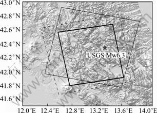
Fig. 1 Shaded relief map of epicenter area (Star represents USGS position of epicenter; Dashed line represents frame of ASAR ascending images; Thin solid line represents frame of ASAR descending images; Thick solid line presents frame of PALSAR images)

Table 1 Details of ASAR images

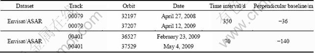
Table 2 Details of PALSAR images

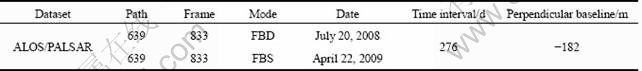
Figures 2(a) and 2(b) show that there are more fringes in ASAR interferogram than in the PALSAR one. The reason is that the longer the wavelength, the less the sensitivity to ground deformation [23]. All of the InSAR data can provide displacement information along their LOS directions, and due to the small incident angles, the ASAR measurements are more sensitive to vertical displacement. From the interferograms, we can see that the main subsidence area lies in the south-west of the earthquake area, with the largest subsidence reaching 0.253 m, 0.192 m and 0.337 m, respectively. The uplift area lies in the north-east of the earthquake area, with the maximum uplift of 0.088 m, 0.050 m and 0.122 m, respectively, in these interferograms. All results are in very good consistency with the results of previous studies [8]. The coseismic displacement field is asymmetric and the subsidence area is approximately 1.5 times the uplift area. Most of the deformation is within a rectangular area of 40 km×30 km.

Fig. 2 Coseismic interferograms of L’Aquila earthquake (Star represents USGS position of epicenter): (a) ASAR ascending (track 401) interferogram; (b) ASAR descending (track 079) interferogram; (c) PALSAR ascending interferogram

2.3 InSAR data reduction

If all these three InSAR deformation data were used in the inversion, the number of observed points would reach 10⁶. This would affect the efficiency of calculation significantly. In order to improve this situation, the down-sampling quadtree algorithm [24] was applied with a reasonable threshold. After the quadtree processing, the pixel points, whose coherence was lower than 0.3 and height difference between epicentral area and observed point was larger than 2 km, were masked out. At the end, the number of InSAR data points was reduced to 1 299.

3 Modeling

To estimate the spatial slip distribution along the fault of the L’Aquila earthquake with the surface displacements, an inverse model is needed. From the geodetic data of InSAR and GPS, the surface rupture was not found in the L’Aquila earthquake area. The fault strike and length cannot be determined by physical method. So this inverse process included two steps. Firstly, the fault geometric parameters were determined using non-linear inversion method based on the model of rectangular dislocation in a homogeneous elastic half space. Secondly, the details of fault slip distribution were inverted using linear inversion method based on a realistic layered crustal structure model with layered characters of L’Aquila area.

3.1 Determining fault geometric parameters

The fault was assumed as a finite uniform slip fault. If the fault dislocation parameters including fault location, strike, dip, slip, rake, length, width and depth were known, then the three-dimensional displacement data could be simulated based on the Okada’s simple homogeneous model [16]. For InSAR data, the simulated three-dimensional deformation can be projected to the LOS direction deformation based on the SAR imaging geometry [25]:

                                   (1)

where d_L is the LOS deformation, θ is the incidence angle of SAR, α is the orientation of the satellite track heading direction, and d_u, d_n and d_e are the three-dimensional deformation upward, north and east, respectively.

From the Okada’s formulae, the relationship between the dislocation parameters and the simulated deformation is non-linear, so a non-linear algorithm is introduced when inverting the fault geometric parameters. Genetic algorithm [26] is a heuristic global search algorithm based on the natural selection and genetic evolutionary ideas, and is used in many engineering fields like geophysical inversion, image processing, and adaptive control. Due to the advantages not affected by the original values, no needs of the objective function derivation and high search speed, the genetic algorithm is suitable for solving this non-linear inversion problem. Since different observations have different contributions to the inversion, their weights should be determined. Here, it is assumed that the ASAR LOS, PALSAR LOS and GPS three-dimensional observations have accuracies of 15, 45, 3, 3 and 6 mm in empirical ratio, respectively. The objective function is a weighted L2-norm of the residuals:

         (2)

where n is the number of observations, p_i and d_i are the weighted ratio and the value of each point observation, f is the function of modeled displacement in observational direction at the point (x_i, y_i), and v is the vector of the fault dislocation parameter.

The non-linear joint inversion was carried out to determinate all the nine fault parameters. Assuming that the Poisson ratio of the model is 0.25, the best fit solution is obtained and is listed in Table 3.

Table 3 Inversed uniform slip fault parameters

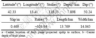
This fault geometric solution shows that the fault is a normal fault with slight right-lateral strike slip. The inverted fault geometry has the same typical characters as the Apennines belt faults, which are normal with NW striking and about 40°-50° dipping. The fault top is   2.5 km lower than the surface. If the fault extends and outcrops to the surface along the updip direction, the surface strike direction and rupture location correspond to the previous rupture of Paganica fault [6]. The strike and dip direction are also similar to the previous studies of fault geometric parameters [1], and the INGV reports [5]. The geodetic moment is M₀=3.23×10¹⁸ N·m (Mw 6.27), assuming that the elastic rigidity μ is 30 GPa as suggested by the previous researchers [3, 20]. The total moment is also similar to the USGS and CMT (3.4×10¹⁸ N·m). So, these geometric parameters can be used to define the fault plane geometry status.

3.2 Layered elastic half-space model

The dislocation model in elastic homogeneous half-space is always used to simulate the surface displacements and to inverse the causative fault dynamic characters. But in this simple analytical solution model, the vertical layered structure character is not included. The influence of this layered character on the simulated deformation has been proved by WANG [19] and it should be considered. To calculate the elastic surface deformation in layered half-space, the most important step is to determinate the kernel functions. The propagator algorithm was used to compute the kernel functions. The solutions of this method are always instable until WANG [18] proposed a simple orthonormalization method. The EDGRN/EDCMP [19] and PSGRN/PSCMP [27] software based on this method are widely used for calculating the static deformation in layered half-space.

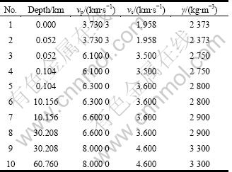
To estimate the fault slip distribution based on the layered half-space model, the first step was to define the parameters of layered media. A new Global Crustal Model of CRUST2.0, which was specified on a 2×2 degree grid, was used to establish the media characters, including density and seismic velocities in the L’Aquila area. The parameters are listed in Table 4. Then, the layered half-space model was set up.

Table 4 Layered crustal structure parameters of L’Aquila area

3.3 Non-uniform slip model inversion

Before inversion of the slip distribution, the fault plane was extended to 16 km×16 km, and divided into  1 km×1 km fault patches along strike line and down-dip direction. The strike and dip direction of every segment was fixed to 139.33° and 50.24°, respectively. After fixing the fault geometric parameters, the inversion of the slip distribution became a linear problem. To solve it, a steepest descent method was employed. Six different direction datasets of the three-dimensional GPS datasets and three InSAR datasets were used to constrain this inversion.

A function of the weighted sum of the squared residual was designed to estimate the fitting effect between the observations and the simulations. The weighted method described in Section 3.1 was used to determine the relative weight ratio for all these six datasets. In inversion process, the goal is to find the best slip distribution solution that can minimize the function. The mathematical formulation is expressed as

  (3)

where U is fault slip vector; d_i (i=1, 2,…, 6, denoting the GPS north, east, vertical and the three different InSAR LOS displacement observations) is the matrix of six observations; d_i⁰ is the static offset of the corresponding observation; p_i is the weighted ratio vector of six datasets; G_i is the Green function for layered elastic half-space, which is the relationship between the observation and prediction; β² is the ratio of smoothing; L is the Laplacian operator; ||L·U||² is defined as the slip roughness.

After more than one thousand iterations, the minimization of Eq. (3) gradually became stable, and the best fault non-uniform slip distribution was achieved. The inverted slip distribution of strike, dip direction and net slip are shown in Fig. 3.

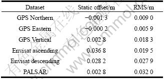
The surface displacements simulated by the best-fit slip distribution model are similar to the observed ones and the root mean square errors between them are listed in Table 5. The histograms of the residual of six datasets for the joint inversion are shown in Fig. 4.

From Table 5 and Fig. 4, we can see that the residuals of the higher accuracy GPS data are the smallest and close to zero. The residuals of InSAR are a little larger, especially those of the PALSAR. These show that the predicted surface displacements using the best-fit slip model are consistent with the observed ones.

The slip over the fault is mainly downdip slip, where most dip slips occur in the central area of the fault, and most of strike slips are concentrated at the top right corner of the fault. These imply that the causative fault is a normal fault with slight right-lateral strike slip. Assuming that the shear modulus is 30 GPa, the total seismic moment is 3.34×10¹⁸ N·m (Mw6.28), slightly lower than 3.4×10¹⁸ N·m estimated by the CMT and USGS. The maximum net slip is about 1.01 m and located in the depth of 8.28 km, similar to the CMT and USGS estimated value 8.8 km, and the rake corresponding to the maximum slip is -96.03°.

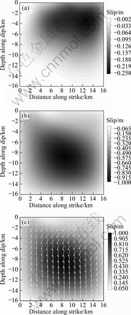
Fig. 3 Slip distribution over L’Aquila fault for layered crustal model: (a) Strike slip; (b) Dip slip; (c) Net slip and rake (Arrows indicate rake direction and magnitude of net slip)

Table 5 RMS of six dataset residuals between observation and simulation

4 Discussion

Because this earthquake is in moderate magnitude, the surface coseismic displacements are not serious and the coherence of interferograms in most L’Aquila area maintains well. Especially in the ALOS/PALSAR differential interferogram, the coherence is good enough to get clear and continuous interferometric fringes. But for the ASAR differential interferograms, the decorrelation in higher mountainous region is considerably serious due to the ground covering, and the ASAR interferometric fringes in these regions are not continuous and will result in low accuracy. In the process of source parameter inversion, the observations in low coherence region are not included.

During the time interval between the acquisitions of selected SAR images used for the coseismic displacement, many foreshocks and aftershocks happened. These aftershocks include the largest shock of 7 April Mw5.6 aftershock. So, the coseismic differential interferograms must contain the information of foreshocks and aftershocks. However, the LOS displacements of these shocks are small enough to be ignored [3]. The coseismic differential interferograms are thought only including the main shock displacement.

The layered character has little influence on the solution of the source parameter inversion under the uniform model, so these parameters can be derived based on the homogeneous elastic half-space model in nonlinear inversion. The result of fault spatial character implies that L’Aquila fault is a NE-SW normal fault and a slight right-lateral fault. The fault of this event belongs to the Paganica normal fault system, whose strike direction is thought to be 130°-140° [28]. The fault strike direction of 139.33° estimated in this work is pretty consistent with the Paganica fault system character and also similar to the result of ANZIDEI et al [1]. The dip result is very close to the fault dip of CHELONI et al [20] and INGV [2] and equivalent to the CMT solution. These show that the geometric parameters define the fault plane well.

The inferred coseismic slip distribution using layered half-space model qualitatively agrees with the seismological model of LIU et al [29], as well as the results of FENG [30] et al and ANZIDEI et al [1]. Assuming the rigidity modulus of 30 GPa, the preferred solution has a total seismic moment of 3.34×10¹⁸ N·m (Mw6.28), which is more close to the CMT and USGS solutions than previous researches. These imply that the layered half-space model can reflect the precise relationship between the fault slip and the surface deformation, and the layered character should be considered in the source parameter inversion.

A simple method was used to determine the weighted ratio among these six different datasets. Nevertheless, it may not be realistic and cannot describe the exact contribution to the inverse model. So, a more reasonable method that can reflect their contribution to the inverse model should be considered in resolving the fault slip distribution.

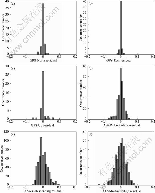
Fig. 4 Histograms of residual between observed and modeled deformation for six datasets

5 Conclusions

1) Ascending orbit PALSAR data, ascending and descending orbit ASAR data were used to obtain the L’Aquila earthquake surface deformation based on the InSAR technique. From three interferograms, the LOS deformation in subsidence area is within 0.337 m, and in uplift area it is within 0.122 m.

2) Based on the elastic homogeneous half-space model and with the InSAR and GPS data constraints, the fault geometric parameters are inverted using the genetic algorithm. The causative fault is almost pure normal mechanism with a small right-lateral component, and the strike and dip angles are 139.33° and 50.24°, respectively.

3) The steepest descent algorithm is employed to inverse the non-uniform slip distribution from different geodetic data based on the crust layered model. The best-fit solution shows that the maximum slip is located in depth of 8.28 km, and total seismic moment is about 3.34×10¹⁸ N·m, which corresponds to Mw6.28.

Acknowledgments

We thank Dr. WANG Rong-jiang for his advice and help in this study. Thanks to European Space Agency (ESA) for its Enviat/ASAR data free of charge used in this work and the precise orbit data povided by the ESA under catergory 1 user projects (No.6994). The ALOS/PALSAR data were provided by the Japan Aerospace Exploration Agency under Project (No.AO-430).

References

[1] ANZIDEI M, BOSCHI E, CANNELLI V, DEVOTI R, ESPOSITO A, GALVANI A, MELINI D, PIETRANTONIO G, RIGUZZI F, SEPE V, SERPELLONI E. Coseismic deformation of the destructive April 6, 2009 L'Aquila earthquake (central Italy) from GPS data [J]. Geophysical Research Letters, 2009, 36: L17307.

[2] Istituto Nazionale di Geofisica e Vulcanologia (INGV). Measurement and modeling of co-seismic deformation during the L'Aquila earthquake, preliminary results [R]. Rome: National Earthquake Center of Italy, 2009.

[3] ATZORI S, HUNSTAD I, CHINI M, SALVI S, TOLOMEI C, BIGNAMI C, STRAMONDO S, TRASATII E, ANTONIOLI A, BOSCHI E. Finite fault inversion of DInSAR coseismic displacement of the 2009 L'Aquila earthquake (central Italy) [J]. Geophysical Research Letters, 2009, 36: L15305.

[4] LI Li, CHEN Yong. Light of earthquake prediction: Shocks before the L'Aquila earthquake of April 6, 2009 [J]. Earthquake Research in China, 2009, 25(2): 151-158. (in Chinese)

[5] Istituto Nazionale di Geofisica e Vulcanologia (INGV). The L'Aquila seismic sequence-April 2009 [R]. Rome: National Earthquake Center of Italy, 2009.

[6] Emergeo Working Group. Geological surveys of the 6 April 2009 L’Aquila seismic sequence epicenter area [R]. INGV report. Ist Rome: National Earthquake Center of Italy, 2009. (in Italian)

[7] PINO N A, LUCCIO F D. Source complexity of the 6 April 2009 L'Aquila (central Italy) earthquake and its strongest aftershock revealed by elementary seismological analysis [J]. Geophysical Research Letters, 2009, 36: L23305.

[8] PAPANIKOLAOU I D, FOUMELIS M, PARCHARIDIS I, LEKKAS E L, FOUNTOULIS I G. Deformation pattern of the 6 and 7 April 2009, MW=6.3 and MW=5.6 earthquakes in L'Aquila (Central Italy) revealed by ground and space based observations [J]. Natural Hazards and Earth System Sciences, 2010, 10: 73-78.

[9] GABRIEL A K, GOLDSTEIN R M, ZEBKER H A. Mapping small elevation changes over large areas: Differential radar interferometry [J]. Journal of Geophysical Research B, 1989, 94(7): 9183-9191.

[10] MASSONNET D, ROSSI M, CARMONA C, ADRAGNA F, PELTZER G, FEIGL K, RABAUTE T. The displacement field of the Landers earthquake mapped by radar interferometry [J]. Nature, 1993, 364: 138-142.

[11] LIU Guo-xiang, DING Xiao-li, LI Zhi-lin, LI Zhi-wei, CHEN Yong-qi, YU Shu-beih. Pre- and co-seismic ground deformations of the 1999 Chi-Chi, Taiwan earthquake, measured with SAR interferometry [J]. Computers & Geosciences, 2004, 30: 333-343.

[12] FUNNING G J, PARSONS B, WRIGHT T J, JACKSON J A, FIELDING E J. Surface displacements and source parameters of the 2003 Bam (Iran) earthquake from Envisat advanced synthetic aperture radar imagery [J]. Journal of Geophysical Research, 2005, 110: B09406.

[13] TONG Xiao-peng, SANDWELL D T, FIALKO Y. Coseismic slip model of the 2008 Wenchuan earthquake derived from joint inversion of interferometric synthetic aperture radar, GPS, and field data [J]. Journal of Geophysics Research, 2010, 115(B04314): 1-19.

[14] ZHANG Hong, WANG Chao, LIU Zhi. The differential radar interferometry technique to achieve coseismic displacement field of the Zhangbei earthquake [J]. Journal of Image and Graphics, 2000, 5(6): 497-500. (in Chinese)

[15] OKADA Y. Surface deformation due to shear and tensile faults in a half-space [J]. Bulletin of the Seismological Society of America, 1985, 75(4): 1135-1154.

[16] TAN Hong-bo, SHEN Chong-yang, XUAN Shong-bai. Influence of crust layering and tickness on coseismic effects of Wenchuan earthquake [J]. Journal of Geodesy and Geodynamics, 2010, 30(4): 29-35. (in Chinese)

[17] XU Cai-jun, LIU Yang, WEN Yang-mao, WANG Rong-jiang. Coseismic slip distribution of the 2008 Mw 7.9 Wenchuan earthquake from joint inversion of GPS and InSAR data [J]. Bulletin of the Seismological Society of America, 2010, 100(5B): 2736-2749.

[18] WANG Rong-jiang. A simple orthonormalization method for stable and efficient computation of Green's functions [J]. Bulletin of the Seismological Society of America, 1999, 89(3): 733-741.

[19] WANG Rong-jiang. Computation of deformation induced by earthquake in a multi-layered elastic crust-FORTRAN programs EDGRN/EDCMP [J]. Computers & Geosciences, 2003, 29: 195-207.

[20] CHELONI D, D'AGOSTINO N, D'ANASTASIO E, AVALLONE A, MANTENUTO S, GIULIANI R, MATTONE M, CALCATERRA S, GAMBINO P, DOMINICI D, RADICIONI F, FASTELLINI G. Coseismic and initial post-seismic slip of the 2009 Mw 6.3 L'Aquila earthquake, Italy, from GPS measurements [J]. Geophysical Journal International, 2010, 181: 1539-1546.

[21] LI Zhi-wei, DING Xiao-li, HUANG Cheng, ZHU Jian-jun, CHEN Yan-ling. Improved filtering parameter determination for the goldstein radar interferogram filter [J]. ISPRS Journal of Photogrammetry & Remote Sensing, 2008, 63: 621-634.

[22] LI Zhi-wei, DING Xiao-li, ZHU Jian-jun, ZOU Zheng-rong. Quantitative study of atmospheric effects in spaceborne InSAR measurements [J]. Journal of Central South University of Technology, 2005, 12(4): 494-498.

[23] JIANG Mi, DING Xiao-li, LI Zhi-wei, ZHU Jian-jun, YIN Hong-jie, WANG Yong-zhe. Study on coseismic deformation of Wenchuan earthquake by use of land C waveband of SAR data [J]. Journal of Geodesy and Geodynamics, 2009, 29(1): 21-26. (in Chinese)

[24] JONSSON S, ZEBKER H, SEGALL P, AMELUNG F. Fault slip distribution of the 1999 Mw7.1 Hector Mine, California, earthquake, estimated from satellite Radar and GPS measurements [J]. Bulletin of the Seismological Society of America, 2002, 92(4): 1377-1389.

[25] HANSSEN R F. Radar interferometry: Data interpretation and error analysis [M]. Dordrecht: Kluwer Academic Publishers, 2001: 162-163.

[26] HOLLAND J H. Adaptation in the natural and artificial systems [M]. Michigan: University of Michigan Press, 1975: 1-10.

[27] WANG Rong-jiang. PSGRN/PSCMP-A new code for calculating co- and post-seismic deformation, geoid and gravity changes based on the viscoelastic-gravitational dislocation theory [J]. Computers & Geosciences, 2006, 32: 527-541.

[28] BONCIO P, PIZZI A, BROZZETTI F, POMPOSO G, LAVECCHIA G, NACCIO D D, FERRARINI F. Coseismic ground deformation of the 6 April 2009 L’Aquila earthquake (Central Italy, Mw6.3) [J]. Geophysical Research Letters, 2010, 37: L06308 .

[29] LIU Chao, XU Li-sheng, CHEN Yun-tai. Quick moment tensor solution of the 2009 April 6, L’Aquila, Italy earthquake [J]. Acta Seismologica Sinica, 2009, 31(4): 464-466. (in Chinese)

[30] FENG Wan-peng, LI Zhen-hong, LI Chun-lai. Optimal source parameters of the April 2009 Mw 6.3 L’Aquila, Italy earthquake from InSAR observations [J]. Progress in Geophysics, 2010, 25(5): 1550-1559. (in Chinese)

(Edited by YANG Bing)

Foundation item: Projects(40974006, 40774003) supported by the National Natural Science Foundation of China; Project(NCET-08-0570) supported by the Program for New Century Excellent Talents in Chinese Universities; Projects(2011JQ001, 2009QZZD004) supported by the Fundamental Research Funds for the Central Universities in China; Projects(09K005, 09K006) supported by the Key Laboratory for Precise Engineering Surveying & Hazard Monitoring of Hunan Province, China; Project(1343-74334000023) supported by the Graduate Degree Thesis Innovation Foundation of Central South University, China

Received date: 2011-05-12; Accepted date: 2011-09-28

Corresponding author: WANG Yong-zhe, PhD Candidate; Tel: +86-15874285386; E-mail: yongzhe.wang@csu.edu.cn