J. Cent. South Univ. (2012) 19: 443-452

DOI: 10.1007/s11771-012-1023-4

Gaussian process assisted coevolutionary estimation of distribution algorithm for computationally expensive problems

LUO Na(罗娜), QIAN Feng(钱锋), ZHAO Liang(赵亮), ZHONG Wei-min(钟伟民)

Key Laboratory of Advanced Control and Optimization for Chemical Processes of Ministry of Education,

East China University of Science and Technology, Shanghai 200237, China

? Central South University Press and Springer-Verlag Berlin Heidelberg 2012

Abstract: In order to reduce the computation of complex problems, a new surrogate-assisted estimation of distribution algorithm with Gaussian process was proposed. Coevolution was used in dual populations which evolved in parallel. The search space was projected into multiple subspaces and searched by sub-populations. Also, the whole space was exploited by the other population which exchanges information with the sub-populations. In order to make the evolutionary course efficient, multivariate Gaussian model and Gaussian mixture model were used in both populations separately to estimate the distribution of individuals and reproduce new generations. For the surrogate model, Gaussian process was combined with the algorithm which predicted variance of the predictions. The results on six benchmark functions show that the new algorithm performs better than other surrogate-model based algorithms and the computation complexity is only 10% of the original estimation of distribution algorithm.

Key words: estimation of distribution algorithm; fitness function modeling; Gaussian process; surrogate approach

1 Introduction

Evolutionary computations have been widely used in science and engineering applications. However, for many practical optimization problems, fitness evaluations of complex model cost too much time. To increase computational efficiency, the original model is often approximated using surrogate model. With the assumption that surrogate model has the true optimum, the optimization result will converge to the correct solutions [1]. Though many great successes have been achieved, surrogate model assisted evolutionary computation also encountered many challenges. Because the surrogate model is eager to smoothen the local optima of the original fitness function, the global optimum and its location are changed. So it is generally difficult to approximate the original fitness for multi-modal landscapes. Also, it is unclear what level of approximation is accurate enough to achieve the desired results. The global optimum is possible to be changed using coarse approximation, while accurate model will bring large computation. Besides these challenges, it is an art to incorporate the surrogate model with the evolutionary algorithm. In addition, it is well known that the surrogate model should be embedded in almost every stage of evolutionary algorithms but how and when to incorporate the approximate model is uncertain.

Coevolution algorithm has emerged as a mechanism to simplify the search space by projecting it into multiple smaller subspaces, which are searched by a separate population. In these subspaces, multi-modal fitness functions can be approximated by surrogate model easily. During coevolution between multiple populations, an automatic coarseness adjustment of approximation models retains [2]. Furthermore, coevolution algorithm is closely related to the estimation of distribution algorithm which has been proposed as a competitor to traditional sample-based evolution algorithms, by replacing the sample population with distribution estimation [3]. As for environment noise, the predictive variance can be provided by Gaussian process model. Above all, the coevolution scheme combined with estimation of distribution algorithm and Gaussian process surrogate model could provide a solution to these fundamental difficulties faced in many fitness approximation applications. Hence, a new surrogate model assisted evolutionary algorithm named Gaussian process assisted coevolutionary estimation of distribution algorithm   (CEDA-GP) is proposed in this work.

2 Related work

2.1 Coevolution

Coevolution is a phenomenon that two or more populations simultaneously evolve with competitive or/and cooperative motion. As an important supplement of Darwin's theory of evolution, coevolution plays an important role during the course of biological evolution. Similarly, biological coevolution inspires a class of algorithms. The initial idea is extended and results in a new optimization procedure called coevolutionary genetic algorithm (CGA) [4]. This algorithm introduces the explicit modularity and provides an appropriate framework for evolving solutions in the form of co-adapted subcomponents. PANAIT [5] provided the underlying theoretical foundation for a better application of cooperative coevolutionary algorithms.

It is usually considered that coevolutionary algorithms are more suitable for complex tasks than non- coevolutionary methods. Hence, coevolution framework is usually used as the start point of evolutionary algorithms. JANSEN and WIEGAND [6] proposed cooperative coevolution (1+1) evolutionary algorithm and investigated the expected optimization time. BERGH and ENGELBRECHT [7] employed cooperative behavior using multiple swarms to optimize different components of the solution vector cooperatively in coevolution particle swarm optimization. Furthermore, the coevolution architecture is combined with univariate estimation of distribution algorithms [3]. In summary, coevolution algorithm decomposes the problem into subcomponents where the interdependencies among different subcomponents are minimal [8] and automatically implements the divide-and-conquer strategy when solving large and complex problems.

Motivated by the possibility of circumventing the curse of dimensionality inherent in surrogate modeling techniques, coevolutionary search was also used to solve computationally expensive optimization problems with surrogate assisted models. Furthermore, fitness predictor coevolved to reduce fitness evaluation cost and frequency, while maintaining evolutionary progress [2].

2.2 Surrogate models

Many empirical models, such as polynomial function, artificial neural network, radial basis function network and support vector machine are often constructed as surrogate models. Polynomial function is carried out first. Though the quadratic or higher order polynomial functions can appropriately approximate single dimension problems, they are difficult to cope with high dimension multi-modal problems. As a generally used curve fitting method, neural network is also put into the approximation for real problems. However, it is unclear to determine network topology to substitute the original fitness function. Besides, hyperparameters of neural network are not accessible. Radial basis function network is also applied while there is a major difficulty to set the optimum decay parameters. As a machine learning method, support vector machine overcomes the difficulties faced in neural network but it cannot predict the uncertainty of the predictions. Recently, Gaussian process (GP) appears as a promising surrogate model. It approximates arbitrary function landscape without predefining the structure of the model and the hyperparameters can be automatically tuned using a theoretical optimization framework. In addition, GP provides an uncertainty measure in the form of a standard deviation. EL-BELTAGY and KEANE [9], SU [10] and BUCHE et al [11] have tried GP as the approximate model in expensive evolutionary optimization.

Though a variety of methods have been tried, there are some open limitations which are hard to overcome. In essence, surrogate models cannot approximate the entire fitness landscape due to the high dimension, ill distribution and limited number of training samples. Instead, they shift their focuses throughout the evolution for good performance. Among these approximation methods, RBF network and GP methods perform better under multiple modeling criteria.

2.3 Estimation of distribution algorithm

Estimation of distribution algorithm (EDA) is a recently developed evolutionary optimization method. Like other evolutionary algorithms, EDA solves the optimization problem by evolving a population of individuals towards promising zones of the search space. Such an evolution is mainly based on iteration between two steps: selection of fit individuals from the current population and combination of the selected individuals in order to create an offspring population and partially replace the current one. The difference is that EDA does not make use of variation operators in the combination step. Instead, EDA generates the offspring population in each iteration by learning and subsequent simulation of a joint probability distribution for the individuals selected. A general outline of EDA is as follows:

1) Initialize a population of individuals randomly.

2) Select individuals for modeling and elite individuals.

3) Estimate probability density function with the probabilistic model.

4) Sample new individuals from probabilistic model as new population.

5) New population is partially replaced by the elite individuals.

6) Stop if some stopping criterion is reached, else go to step 2).

The use of a probabilistic model is the key concept of any EDA. For combination optimization problems, EDAs use a product of independent univariate probabilities, Bayesian network or other models. In continuous domain, Gaussian model is widely used for its simplicity. Also, hybrid Gaussian model was proposed to compensate the shortage of Gaussian model [12]. Non-parametric histogram model has been used in EDA without any assumption of population distribution [13].

3 Gaussian process assisted coevolutionary estimation of distribution algorithm

3.1 Framework

CEDA-GP begins with the decomposition of the search space. Two populations are used for exploiting the search space. The first population is divided into n sub-vectors to evolve and the second population is evolved in the original process. The initialization of populations is randomly generated as the conventional evolutionary algorithm. The initial individuals are assessed using the original exact fitness function. Subsequently, the algorithm proceeds into the model building phase. Based on GP, a cheap surrogate model is built. In order to verify the accuracy of the model, the original exact fitness of the best individual is compared with the value calculated by the model. If the evolution control criterion is not reached, the model is accepted to be used for the next generation, else the model is  updated. With improved solutions, the algorithm proceeds to estimate the probability density function and reproduce the new population. The search cycle is then repeated until a termination criterion reaches. A brief outline of CEDA-GP is presented in Fig. 1.

3.2 Coevolutionary strategy

Combined with the notion of coevolution, many evolutionary algorithms have been investigated and applied widely [14-15]. In this work, coevolutionary estimation of distribution algorithm (CEDA) performs exploitation by using two kinds of populations. The first population is divided into m sub-vectors using principle component analysis. The complete solution is the vector containing the best sub-vector of each population, as illustrated in Fig. 2. These sub-vectors work sequentially. One sub-vector focuses on evolving the specified variables while other sub-vectors are maintained “frozen”, vice versa. The combination of the m sub-vectors provides the overall solutions. The second population is evolved in the original process. Between the two populations, the first population shares the better solutions which are in the elitism set of the second population and the second population only shares the global best solution of the first population. The decomposing and cooperating process leads to a complete investigation of the search space since the solution is evaluated every time when a single component changes, which implements an exhaustive exploitation of the whole space.

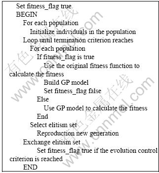
Fig. 1 Algorithm for CEDA-GP

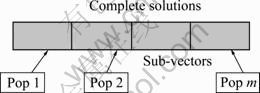
Fig. 2 Solution structure of CEDA

Usually, the coevolution strategy brings complex computation. While in this work, the fitness values of the first population are calculated using the approximation model. In order to make the balance between the accuracy and computation complexity, the best individual in every sub-vector is calculated using the original fitness function. So, the computation is only a little more increased.

3.3 Evolution of populations

The evolution of populations is based on the mechanism of estimation of distribution algorithm. For the two populations, CEDA mainly includes three steps: selection, reproduction and replacement.

3.3.1 Selection operation

Before generating a new population, a subset of solutions is selected into the set D_s and further used for learning phase. In most EDAs, proportional or tournament selection methods are usually used. For example, a truncation selection is often employed in UMDA, where typically 50% best solutions are selected. Different from the traditional EDAs, in the surrogate model for expensive computation problems, the fitness evaluation is usually not the actual value of the original model. So, the selection operation includes two aspects: the model predictions and the standard variance of the predictions. For the original fitness, the standard variance is set as zero. The fitness prediction using GP model is as follows:

                                                            (1)

where  is the fitness value used in CEDA-GP;  is the prediction;  is the standard variance of the prediction; α is the coefficient of the prediction and β is the coefficient of the standard variance, α=0.7, β=0.3. Fitness values are ordered using the value of Eq. (1). Truncation selection is employed based on the new fitness values. The truncation ratio is usually set as 0.3. Similarly, the elitism individuals are selected for replacement and the elitism set is proportional to the population.

3.3.2 Reproduction operation

For the subset of selected promising solutions, probability density is estimated and the new population is generated from the estimated distribution. In CEDA-GP, the sub-vectors in the first population are assumed independent while the second population is the complete vector. Thus, two different probability density models are used in the first and second populations.

For the sub-vectors in the first population, univariate Gaussian model is used to estimate the distribution of the individuals,  As for the estimation of the mean  and the variance , the maximum likelihood is used.  and  are calculated as follows:

                                                             (2)

                                                 (3)

where i is the i-th dimension of the variant; x_i,m is the sample of variant x_i; n is the number of samples;  and  are estimation value of  and  in the current dimension.

For the second population, Gaussian mixture model (GMM) is used to estimate both distribution of variables and the interdependences among them. The model usually takes the formula as follows:

          (4)

where p is the number of Gaussian model and ω_i is the mixing weight; μ_i and Σ_i are the mean and covariance matrix in the Gaussian model. For the estimation of parameters ω_i, μ_i and Σ_i, expectation maximization (EM) algorithm is usually used.

In order to reproduce new populations, different sampling methods are used. New individuals of the first population are sampled using the mean and variance from a univariate Gaussian model, while the second population generates samples from a mixture of full multivariate Gaussian models.

3.3.3 Replacement operation

From the previous generation of the two populations, elitisms are preserved in the sense that all selected solutions are reserved in every generation. After generating a set of new individuals, a new population is created by replacing some individuals with the elitisms. Alternatively, the selected elitisms replace a fraction of the selected population from the previous generation rather than the entire population. So, the population can reserve the promising solutions during the evolution.

3.4 Model building

In CEDA-GP, surrogate model is built using Gaussian process. There are three steps to train and update the GP model.

3.4.1 Hyperparameters estimation of GP model

A global model usually gives a rough estimation of a function over a large domain, while a local model gives a more precise estimate over a smaller sub-domain. In order to compromise between global models and local models, sampling strategy should be determined.

In CEDA-GP, a prior assumption is stated that the distribution of data is the Gaussian mixture distribution. Therefore, individuals are located in the interesting regions. The sampling of data which is used in CEDA-GP is automatically selected. During the initialization, new samples are taken from the true fitness function and the samples are made up of individuals in the first and the second population. During the evolution, individuals in the second population and the elitism set in the first population consist of the samples. The GP model is therefore rebuilt when evolution control criterion is reached. By periodically updating the model to introduce new information and refining it around the promising areas of the search space, the GP model becomes better interpreted with a global approximation and more precise in some interesting regions.

For l data points  it is assumed that the target values t_i can be obtained from the corresponding function value y_i by means of additive Gaussian noise ε (t_i=y_i+ε,  So, GP can be expressed as a collection of random variables with joint multivariate Gaussian distribution (y₁, …, y_l)N(0, K), where K is the l×l covariance matrix with entries K^ij=k(x_i, x_j). In GP, covariance function k(x_i, x_j) is a parameterized function from pairs of x values to their covariance. One common form of covariance function is d dimensions squared exponential covariance function:

           (5)

where x_i and x_j are the i-th and j-th vectors in the population separately, x_i,m and x_j,m are the m-th dimension value of x_i and x_j. v₀ and λ_m (m=1, …, d) are hyperparameters, v₀ specifies the overall y-scale and λ_m is the length-scale associated with the m-th coordinate.  is a “jitter” term, which is added to prevent ill-conditioning of the covariance matrix of the outputs.

In order to estimate hyperparameters of covariance function, the log likelihood is usually used. The log likelihood of the vector y under a Gaussian process with mean 0 and covariance  is

   (6)

where Θ is hyperparameter and Θ=[υ₀, λ₁, …, λ_d]. In order to get the solution of Θ, it is necessary to calculate the derivatives of L with respect to hyperparameters Θ:

        (7)

When the derivative functions are equal to zero, the solution of hyperparameters Θ can be solved. For a new test input x^*, given the assumption of a Gaussian process prior over functions, it is a standard result that the predictive distribution p(y^*|x^*, X, y) is

                                     (8)

where

                                      (9)

        (10)

The covariance matrix k(x^*) satisfies k(x^*)=K(X, x^*).  gives the error bars or confidence interval of the prediction.

Compared with other modeling methods, the advantage of GP is that it can give the predictive error for the solutions. Just as Fig. 3 shows, GP is used to model single dimension function y=chol(k(x, x′)) with white noise of 0.89. The covariance function is selected as k(x, x′)=v₀exp[-(x-x′)Σ^-1(x-x′)′/λ]. With data points (circles in Fig. 3), parameters are optimized to v₀=3.0, λ=1.16. GP model is the black curve and the error bar is around the curve in shadow. It is obvious that the error bar is narrow when the data points are dense, and vice versa. In summary, GP can give the value and variance of the predictions. Based on this character, it is often used for modeling, especially for soft sensor modeling [16].

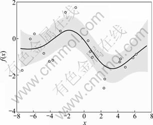
Fig. 3 GP model for chol function

3.4.2 Model update

Though the use of surrogate models for fitness evaluations may reduce the number of fitness evaluations significantly, the application of surrogate models to evolutionary computation is not as straightforward as expected [17]. The evolutionary algorithm is easy to converge to a false optimum which is an optimum of the surrogate model, but not that of the original fitness function. In order to avoid the occurrence of such cases, evolutionary control is used in this work.

Evolutionary control is regarded as the issue of model management and it provides the ratio between the used surrogate models and the original fitness function. It is intuitive that the higher the fidelity of the surrogate model, the more often the fitness evaluation can be made using the model. However, it is very difficult to estimate the global fidelity of the surrogate model. JIN et al [1] used the current model error to estimate the local fidelity of the surrogate model and then to determine the frequency at which the original fitness function is used and the approximate model is updated. However, it is not easy to realize it in reality.

There are two kinds of evolutionary control strategies: fixed evolution control and adaptive evolution control. For fixed individual or generation evolution control, the frequency of approximate model is constant. The drawback of this strategy is the strong oscillation during optimization due to large model errors. But in many complex multi-dimension problems, good performance can be obtained with appropriate control frequency of generation. Adaptive evolution control adjusts the frequency of evolution control based on the trust region framework.

In order to compromise between simplicity and accuracy of surrogate model, the two evolution control strategies are tested using Rosenbrock benchmark function. The comparison is shown in Fig. 4. It is clear that with suitable fixed generation control, the optimization can proceed as the same as the algorithm with adaptive evolution control. It is difficult for the algorithm to converge when the approximate model is of low fidelity.

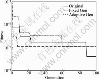
Fig. 4 Influence of evolution control strategies

4 Numerical examples

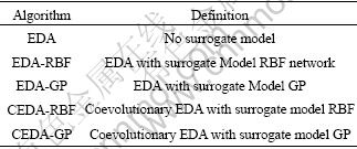
Empirical study on CEDA-GP is performed using 6 benchmark problems (F₁-F₆) with detailed descriptions provided in Appendix A. These problems are multi- modal and continuous. In addition, they are configured with a dimension d=10. Performance comparisons are then made between EDA, EDA-RBF, EDA-GP, CEDA-RBF and CEDA-GP (refer to Table 1 for the definition of the algorithms investigated here). Note that to facilitate a fair comparison, the surrogate variants are built on top of the same EDA used in the study, which ensures that any improvement observed is a direct contribution of the surrogate framework considered.

Table 1 Definitions of algorithms compared

The algorithms are employed with population size of 300, truncation coefficient of 0.3, elitism individuals in each generation of 30 and the maximum number of iteration of 100 iteratively. At each 5 search generations, the algorithms employ RBF neural network or GP surrogate model to screen the entire population of individuals. In order to guarantee the fitness of the samples not far from real value, the best fitness individuals in the population undergo exact evaluations.

In order to compare the algorithms, three different criteria are used, which are the convergence ability, the computation complexity and the validation of surrogate models.

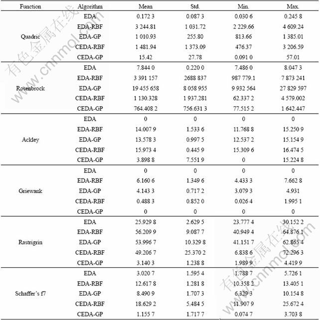
4.1 Convergence ability

In order to analyze the convergence ability, we focus on the critical solutions obtained by CEDA-GP and other algorithms. Twenty independent consecutive experiments are conducted to find the optimum. Statistical results of the independent experiments are listed in Table 2. It can be seen from Table 2 that CEDA-GP outperforms other algorithms in most benchmark functions. For Quadric benchmark function, only one optimum exists but the interdependence added makes it difficult to find global optimum. Though CEDA-GP can find better solutions than EDA-RBF, EDA-GP and CEDA-RBF, this surrogate algorithm is difficult to have the same performance as using the original fitness function. For Rosenbrock benchmark function, CEDA-GP cannot yet find the optimum solutions as EDA. While in other benchmark functions, CEDA-GP appears good or even better than EDA. Other algorithms such as EDA-GP, EDA-RBF and CEDA-RBF still cannot converge to the global optimum as EDA and CEDA-GP. This illustrates that for some problems especially with unimodal property, surrogate models should be applied with caution. Because the surrogate models may change the global optimum of the original fitness model, more original fitness estimations should be used during the optimization. For multi-modal optimization problems, GP can reconstruct the curve of the original fitness with samples provided by CEDA and GP-CEDA can find the global optimum companied.

In order to clearly illustrate the convergence ability of CEDA-GP, an evolutionary course of the global best fitness evaluations for each algorithm was randomly selected. The results are shown in Fig. 5. It is obvious that in most benchmark functions, CEDA-GP performs significantly better than EDA-RBF, EDA-GP and CEDA-RBF. For special benchmark functions such as Ackley with too many closely local optima, the evolutionary course of CEDA-GP is worse than EDA-RBF. Because the algorithms are stochastic and heuristic, the run is randomly selected and the result can be adopted. Compared with the original EDA with true fitness function, CEDA-GP can find better solutions in some cases. This indicates that the surrogate model in CEDA-GP can smoothen the local optima of the original multi-modal fitness function without changing the global optimum and its location.

4.2 Computation complexity

For expensive computation problems, fitness function evaluation costs a lot of time. In comparison with the time of evaluating the original fitness function, the evolving time of EDA and CEDA is much shorter.  So, the computation complexity is defined as the number of calculating the original fitness functions. As for the original EDA without surrogate model, the number of original fitness evaluation with 300 population and 100 generation is 30 000. While EDA-RBF and EDA-GP where surrogate models are updated every five generations need 6 000 times of fitness evaluation. In CEDA-RBF and CEDA-GP, the model is updated using the selection sets in the second population and the elitism individuals in the first population on an interval of five generations. Both of two algorithms only need 3 300 times to calculate the original fitness function. The comparisons of computation complexity among these algorithms are shown in Fig. 6. It is illustrated that with coevolution algorithms, the computation complexity of CEDA-GP is decreased. Only with the quality of GP model, fewer samples can provide interesting regions for CEDA to optimize.

Table 2 Performance comparison between different algorithms

4.3 Validation of surrogate models GP

The accuracy of surrogate model is critical during the evolution course. So in this section, the approximation performance of surrogate models is empirically investigated. For simplicity, the investigation is carried out on 2-D Rosenbrock function with GP and RBF neural network model under CEDA.

In every five runs of evolution, the individuals are generated with the 2-D Rosenbrock fitness function. Therefore, among the period, the middle run to validate the surrogate models is chosen. The fitness values estimated from GP and RBF network are shown in Fig. 7. Compared with the true 2-D Rosenbrock function, it is seen that the approximation of GP is more accurate than that of RBF network. At the beginning of the evolution, GP model automatically tunes the hyperparameters and the range of the approximation is wide but close to the true fitness. While for RBF  network, many points of the model are far from the true fitness. With evolution going on, the optimization range decreases. GP model can simulate the shape of the true 2-D Rosenbrock function while RBF network has serious errors.

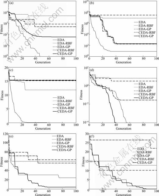
Fig. 5 Solutions of CEDA-GP compared with EDA, EDA-RBF, EDA-GP, CEDA-RBF with different benchmark functions:       (a) Quadric; (b) Rosenbrock; (c) Ackley; (d) Griewank; (e) Rastrigin; (f) Schaffer’s f7

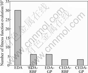
Fig. 6 Computation complexity of CEDA-GP and other algorithms

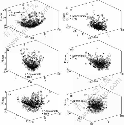
Fig. 7 Fitness evaluations compared between GP and RBF network during evolutionary course of CEDA-GP and CEDA-RBF:     (a) GP model, iter=3; (b) RBF model, iter=3; (c) GP model, iter=7; (d) RBF model, iter=7; (e) GP model, iter=17; (f) RBF model, iter=17

From evolutionary course of algorithms CEDA-GP and CEDA-RBF, GP model displays better approximation performance than RBF network. That is because the initial parameters of RBF network influence the fitting and generalization performance. With randomly selected parameters and predefined structure, RBF network is not well trained. But for GP, the hyperparameters are tuned automatically and it does not need to preset the initial parameter values. Also, the populations in CEDA provide Gaussian mixture distribution, which makes the GP model more precise. From the experience, it is clear that CEDA-GP is apt to converge to the global optimum.

5 Conclusions

1) A novel optimization algorithm CEDA-GP for accelerating expensively computational problems is presented. Different from other algorithms, coevolutionary idea helps the surrogate model approximate multi-modal fitness landscapes and automatically determines the level of approximation.

2) The algorithm CEDA-GP makes use of both the advantages of GP surrogate model and excellent global search capability of CEDA to find the promising individuals during searching process for the global optimum solution.

3) Experimental studies are presented to validate the feasibility of CEDA-GP. The proposed optimization framework of CEDA-GP is capable of solving computationally expensive optimization problems and can clearly outperform surrogate algorithms using neural network model on a limited computational budget.

Appendix A: benchmark functions

Quadric:

-100≤x_i≤100, i=1, …, n

Global optimum x^*=(0, …, 0)_n, f(x^*)=0

Rosenbrock:

-50≤x_i≤50, i=1, …, n

Global optimum x^*=(1, …, 1)_n, f(x^*)=0

Ackley:

-30≤x_i≤30, i=1, …, n

Global optimum x^*=(0, …, 0)_n, f(x^*)=0

Griewank:

-300≤x_i≤300, i=1, …, n

Global optimum x^*=(0, …, 0)_n, f(x^*)=0

Rastrigrin:

-5.12≤x_i≤5.12, i=1, …, n

Global optimum x^*=(0, …, 0)_n, f(x^*)=0

Schaffer’s f7:

-100≤x_i≤100, i=1, …, n

Global optimum x^*=(0, …, 0)_n, f(x^*)=0

References

[1] JIN Yao-chu, OLHOFER M, SENDHOFF B. A framework for evolutionary optimization with approximate fitness functions [J]. IEEE Transactions on Evolutionary Computation, 2002, 6(5): 481-494.

[2] SCHMIDT M D, LIPSON H. Coevolution of fitness predictors [J]. IEEE Transactions on Evolutionary Computation, 2008, 12(6): 736-749.

[3] VO C, PANAIT L, LUKE S, Cooperative coevolution and univariate estimation of distribution algorithms [C]// Proceedings of the 10th ACM SIGEVO Conference on Foundations of Genetic Algorithms, Association for Computing Machinery. Orlando, Florida, USA: 2009: 141-150.

[4] POTTER M A, DEJONG K A. A cooperative coevolutionary approach to function optimization [C]// DAVIDOR Y, SCHWEFEL H, M?NNER R. The Third Parallel Problem Solving from Nature. Springer Berlin/Heidelberg, 1994: 249-257.

[5] PANAIT L. Theoretical convergence guarantees for cooperative coevolutionary algorithms [J]. Evolutionary Computation, 2010, 18(4): 581-615.

[6] JANSEN T, WIEGAND R P. The cooperative coevolutionary (1+1) EA[J]. Evolutionary Computation, 2004, 12(4): 405-434.

[7] BERGH F V D, ENGELBRECHT A P. A cooperative approach to particle swarm optimization [J]. IEEE Transactions on Evolutionary Computation, 2004, 8(3): 225-239.

[8] YANG Z Y, TANGA K, YAO X. Large scale evolutionary optimization using cooperative coevolution [J]. Information Sciences, 2008, 178(15): 2985-2999.

[9] EL-BELTAGY M A, KEANE A J. Evolutionary optimization for computationally expensive problems using gaussian processes [C]// Proceedings of the International Conference on Artificial Intelligence. Las Vegas: CSREA Press, 2001: 708-714.

[10] SU Shao-guo. Accelerating particle swarm optimization algorithms using gaussian process machine learning [C]// QI L, TIAN X Z. Proceedings of the 2009 International Conference on Computational Intelligence and Natural Computing. Wuhan: IEEE Computer Society, 2009: 174-177.

[11] BUCHE D, SCHRAUDOLPH N N, KOUMOUTSAKOS P. Accelerating evolutionary algorithms with gaussian process fitness function models [J]. IEEE Transactions on Systems Man and Cybernetics Part C-Applications and Reviews, 2005, 35(2): 183- 194.

[12] LI Bin, ZHONG Rui-tian, WANG Xian-ji, ZHUANG Zhen-quan. Continuous optimization based-on boosting gaussian mixture model [C]// TANG Y Y, WANG S P, LORETTE G, YEUNG D S, YAN H. Proceedings of the 18th International Conference on Pattern Recognition (ICPR 2006). Hong Kong, China: IEEE Computer Society, 2006: 1192-1195.

[13] DING N, ZHOU S, SUN Z. Histogram-based estimation of distribution algorithm: A competent method for continuous optimization [J]. Journal of computer science and technology, 2008, 23(1): 35-43.

[14] KROHLING R A, COELHO L D. Coevolutionary particle swarm optimization using gaussian distribution for solving constrained optimization problems [J]. IEEE Transactions on Systems Man and Cybernetics Part B-Cybernetics, 2006, 36(6): 1407-1416.

[15] ZHAO Liang, YANG Yu-pu, ZENG Yong. Eliciting compact t-s fuzzy models using subtractive clustering and coevolutionary particle swarm optimization [J]. Neurocomputing, 2009, 72(10/11/12): 2569- 2575.

[16] XIONG Zi-hua. Soft sensor modeling based on gaussian processes [J]. Journal of Central South University of Technology, 2005, 12(4): 469-471.

[17] JIN Yao-chu. A comprehensive survey of fitness approximation in evolutionary computation [J]. Soft Computing, 2005, 9(1): 3-12.

(Edited by HE Yun-bin)

Foundation item: Project(2009CB320603) supported by the National Basic Research Program of China; Project(IRT0712) supported by Program for Changjiang Scholars and Innovative Research Team in University; Project(B504) supported by the Shanghai Leading Academic Discipline Program; Project(61174118) supported by the National Natural Science Foundation of China

Received date: 2011-06-21; Accepted date: 2011-10-19

Corresponding author: QIAN Feng, Professor, PhD; Tel: +86-21-64252060; E-mail: fqian@ecust.edu.cn