Trans. Nonferrous Met. Soc. China 26(2016) 1232-1250

Flow stress prediction for hot deformation processing of 2024Al-T3 alloy

D. TRIMBLE, G. E. O’DONNELL

Department of Mechanical & Manufacturing Engineering, Trinity College Dublin, College Green, Dublin 2, Ireland

Received 13 May 2015; accepted 3 April 2015                                                                                              

Abstract: Isothermal compression tests were conducted to predict the hot deformational flow stress behaviour of 2024Al-T3 alloy with respect to a wide range of strain rates (0.001-100 s^-1), strains (0.1-0.5) and temperatures (573-773 K). The prediction capabilities of various constitutive models for 2024Al alloys and a recently developed constitutive model were evaluated using statistical parameters such as the average absolute relative error (AARE) and the correlation coefficient (R). Models recorded the lowest AARE (4.6%) and the highest correlation coefficient (R=0.99) were developed compared with the other models. Hence, this model can track the deformational behaviour of 2027Al-T3 alloy more accurately compared with other models throughout the entire processing domain investigated.

Key words: isothermal compression; 2024Al alloy; constitutive model; flow stress                                                                                                            

1 Introduction

2024 aluminium alloys are used extensively within the aerospace industry to fabricate structural components such as aircraft fuselage and wing panels due to their high strength to mass ratio [1,2]. Finite element (FE) methods have been successfully used to analyze and optimize bulk metal deformation processes [3], metal machining processes [4,5] and solid state joining processing [6] of these aluminium alloys. During the development of a FE simulation, the constitutive model of the workpiece material was used as an input to simulate material deformation behaviour under specified loading conditions [7]. Therefore, the precision of the numerical simulation depends on how accurately the deformation behaviour of the material is represented by the constitutive model [8]. Usually, the constitutive model is a mathematical representation describing the relationship among flow stress, strain, strain rate and temperature [9].

Many constitutive models have been proposed or modified to describe the flow stress behaviour of 2024Al alloys over different ranges of temperatures and strain rates. Table 1 highlights previous research publications in this area. In terms of aluminium alloys, one of the earliest and most common constitutive models is the hyperbolic sine Arrhenius-type model proposed by ZENER and HOLLOMON [10], and SELLARS and TEGART [11]. SHEPPARD and JACKSON [12] performed hot compression and hot torsion tests to determine the flow stress behaviour of 2024Al alloy using this Arrhenius-type model. Hot torsion tests were conducted by CEPEDA-JIMENEZ et al [13] to determine the flow stress behaviour of 2024Al-T351 alloy also using the Arrhenius-type model. More recently, HAO et al [14] used the Arrhenius-type model to establish the flow stress behaviour of 35%SiC_p/2024 aluminium metal matrix composite. A major disadvantage of the Arrhenius model is that the effect of strain is not considered. LIN et al [15] proposed a modified Arrhenius-type model with strain compensation to encapsulate the effect of strain to establish the flow stress behaviour of 42CrMO steel.

The Johnson-Cook model is another example of a well-established constitutive model. JOHNSON and COOK [16] used their proposed model to determine the flow stress behaviour of 2024Al-T351 alloy by performing isothermal and adiabatic torsion tests. LESUER [17] performed high strain rate compression tests on 2024Al-T3 alloy using a split Hopkinson pressure bar (SPHB) system to determine new constants for the Johnson-Cook model. However, SPHB tests at different temperatures were not completed. SEIDT and GILAT [18] performed a number of tension, compression and torsions tests on 2024Al-T351 alloy test pieces at different specimen orientations to determine the flow stress behaviour using the Johnson-Cook model. However, the effect of temperature was investigated at one strain rate only. AMIR et al [19] performed machining investigations based on Ref. [20] to further refine the original constants of the Johnson-Cook model for 2024Al-T351 alloy.                    

Table 1 Highlight of previous research on developing constitutive models for 2024 aluminium alloys

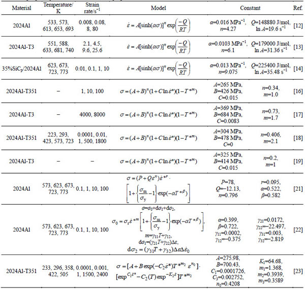
More recent constitutive models have focused on the modification of existing models or the development of new constitutive models. MAHESHWARI et al [21] proposed a modified Johnson-Cook model to describe the flow stress behaviour of 2024Al alloy from experimental compression data. It was found that in most cases, the modified model correlated better with experimental results compared with the original Johnson-Cook model. More recently, MAHESHWARI [22] proposed a new phenomenological constitutive model which correlated even better with experimental data compared with that previously proposed modified Johnson-Cook model [21]. KHAN and LIU [23] performed compression tests on 2024Al-T351 alloy and proposed a new phenomenological model to describe the flow stress behaviour. LIN et al [24] proposed a new constitutive model to predict the hot tensile deformation behaviour of Al-Cu-Mg, Al-Zn-Mg-Cu [25] and 7075Al [26] alloy based on the original Johnson-Cook model. The authors reported greater prediction capability compared with the Johnson-Cook model. TRIMBLE and O’DONNELL [27] have also recently developed a new constitutive model to describe the flow stress behaviour of 7075Al.

The objective of this study was to establish the flow stress behaviour of 2024Al-T3 through isothermal compression tests. This was achieved by evaluating the prediction capability of various constitutive models for 2024Al alloys and a recently developed constitutive model using statistical parameters such as average absolute relative error (AARE) and correlation coefficient (R).

2 Experimental

2024Al-T3 alloy cylindrical specimens with a diameter of 6 mm and height of 9 mm in the extrusion direction were prepared for compression tests from extruded bar stock in accordance with ASTM E209 [28]. The chemical composition of the material is shown in Table 2. The average grain sizes in the extruded direction were 90 μm and 30 μm in the width direction. A Gleeble-3800 mechanical simulator was used to perform isothermal compression tests as shown in Fig. 1(a). The cylindrical specimen was clamped between two compression dies and the deformational temperature was measured by thermocouples welded to the central regions of the specimen surface as shown in Fig. 1(b). To minimise friction, a combination of tantalum foil (thickness of 0.05 mm) and nickel-based lubricant was placed at the interface of the workpiece and heating anvils.  Thirty compression tests were performed over ranges of temperatures (573, 623, 673, 723, 773 K) and strain rates (0.001, 0.01, 0.1, 1, 10, 100 s^-1). Each specimen was heated to the deformation temperature at a rate of 5 K/s by thermo-coupled feedback-controlled AC current using resistive heating. To obtain an equal heat distribution, the specimen was held for 2 min at isothermal conditions before compression. The specimens were plastically deformed to a strain of 0.5 if strain hardening occurs. Figure 2(a) shows the schematic diagram of the heating process. Standard equations were used to convert the load-stroke data to true stress-true strain data as shown in Eqs. (1) and (2), where σ is the true stress, P is the load, A₀ is the original cross-sectional area, e is the engineering strain, ε is the true plastic strain, h₀ is the original height of the specimen and h is the instantaneous height of the specimen. The elastic region was subtracted from the true stress-strain curve to get the true stress-true plastic strain data, which represents the flow stress data required when establishing constitutive models as shown in Fig. 2(b).

σ=P/A₀(1-e)                                 (1)

 

ε=-ln(h₀/h)                                  (2)

Table 2 Chemical composition of experimental 2024Al-T3 alloy (mass fraction, %)

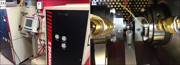
Fig. 1 Gleeble-3800 thermo-simulation machine (a) and compression area (b)

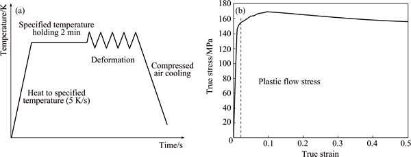
Fig. 2 Schematic diagram of heating process (a) and subtraction of elastic data using 0.2% offset strain (b)

3 Results

3.1 Arrhenius-type model

The effects of temperature and strain rate on deformation behaviour can be represented by the Zener-Holloman parameter (Z) in an exponent-type equation expressed as [10]

                              (3)

where  is the strain rate, R is the mole gas constant, T is the temperature (K) and Q is the activation energy of hot deformation (kJ·mol^-1). The Arrhenius-type model, which gives the relationship between flow stress and Z can be expressed as [11]

                          (4)

where σ is the flow stress (MPa) for a given strain, α, n, A, and Q are material constants (α=β/n₁). In this work, astrain of 0.3 was taken as an example to introduce the solution procedures to determine the material constants. For low stress levels (ασ<0.8) and high stress levels (ασ>1.2), substituting the power law and exponential law of F(σ) into Eq. (4) yields the following:

                                   (5)

 

                               (6)

where B and C are material constants. Taking the natural logarithm of both sides of Eqs. (5) and (6), respectively, gives

                          (7)

 

                            (8)

By substituting the values of flow stress and corresponding strain-rate under the strain of 1.0 for all deformation temperatures into Eq. (10), values for n₁ and β can be calculated from the slope of the plots lnσ against  and σ against  respectively as shown in Figs. 3(a) and (c). The average slope values at the different temperatures are taken when calculating n₁ and β. Then, the corresponding value of α=β/n₁ can be calculated.

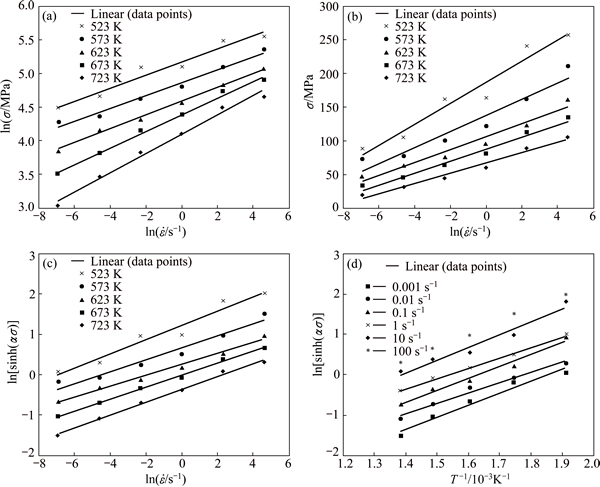
Fig. 3 Plots of ln σ against  (a), ln[sinh(ασ)] against  (b),

 σ against  (c) and ln[sinh(ασ)] against 1000/T at strain of  3.0 (d)

When considering all stress levels, Eq. (9) can be expressed as

 

                    (9)

Taking the natural logarithm of both sides and rearranging, Eq. (9) can be expressed as

               (10)

By substituting the values of flow stress and corresponding strain rate under the strain of 1.0 at all deformation temperatures into Eq. (10), the value for n can be calculated from the average slope in the plot of  ln[sinh(ασ)] against  as shown in Fig. 3(b). By differentiating Eq. (10), the following formula can be derived for a particular strain rate:

                   (11)

The value of Q can be calculated from the average slope of the plot of ln[sinh(ασ)] against 1000/T under different strain rates as shown in Fig. 3(d). Hence, the value of A can be calculated from the intercept of the plot ln[sinh(ασ)] against . The influence of strain on flow stress behaviour is assumed to be insignificant in Eqs. (3) and (4). Hence, it is necessary to use a method of strain compensation. The influence of strain in the constitutive model is incorporated by assuming that the material constants are polynomial functions of strain. A second order polynomial, as shown in Eq. (12), represents the influence of strain on material constants with good correlation and generalisation as shown in  Fig. 4. The coefficients of the polynomial are given in Table 3.

                        (12)

According to the definition of hyperbolic law, the flow stress can be written as a function of the Zener-Hollomon parameter as shown in Eq. (13). The comparison between the experimental and predicted data from the strain compensated Arrhenius-type constitutive model under various processing conditions is shown in Fig. 5.

            (13)

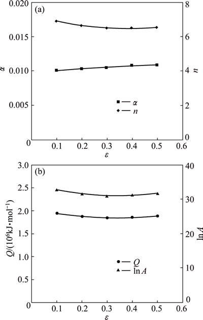
Fig. 4 Variation of α and n (a) and Q and ln A (b) with true strain

Table 3 Polynomial coefficients for α, n, Q and lnA

3.2 Johnson-Cook model

The Johnson-Cook model can be represented as follows [16]:

                (14)

where σ is the flow stress, ε is the plastic strain,  is the dimensionless strain-rate with  being the strain rate and  (1 s^-1) being the reference stain rate, T*=(T-T_ref)/(T_melt-T_ref) with T being the current temperature, T_ref (573 K) being the reference temperature and T_melt (911 K) being the melting temperature. Parameters A, B, C, n, and m are all material constants. At reference temperature and strain rate, and multiplying by the natural logarithm, Eq. (14) can be rearranged to

ln(σ-A)=ln B+nln ε                           (15)

where A is the yield strength at reference temperature and strain rate. B and n can be calculated from the intercept and slope of ln(σ-A) against ln ε respectively as shown in Fig. 6(a) by performing a linear fit. At reference temperature, Eq. (14) can be rearranged to

                        (16)

C can be calculated from the slope of [σ/(A+Bεⁿ)]-1 against  as shown in Fig. 6(b) by performing a linear fit. By multiplying by the natural logarithm  Eq. (14) can be rearranged to

          (17)

m can be calculated from the slope of  against  as shown in Fig. 6(c) by performing a linear fit. Table 4 shows the initial and optimised constants for the JC model. Using these constants, the flow stress data are predicted under various processing conditions. Comparison between the experimental and predicted data by the JC model is shown in Fig. 7.

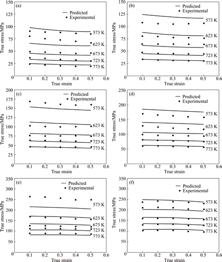
Fig. 5 Comparison between experimental and predicted flow stress values by Arrhenius-type strain compensated model at strain rate of 0.001 s^-1 (a), 0.01 s^-1 (b), 0.1 s^-1 (c), 1 s^-1 (d), 10 s^-1 (e), 100 s^-1 (f)

Fig. 6 Plots of ln(σ-A) against ln ε at reference strain rate and temperature (a) and  against  (b) and   against  (c)

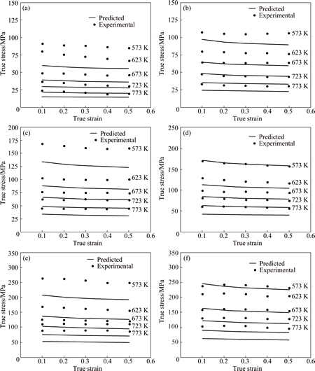
Fig. 7 Comparison between experimental and predicted flow stress values by Johnson-Cook model at strain rate of 0.001 s^-1 (a),  0.01 s^-1 (b), 0.1 s^-1 (c), 1 s^-1 (d), 10 s^-1 (e), 100 s^-1 (f)

Table 4 Constants for Johnson-Cook model

3.3 Modified Johnson-Cook model

The modified Johnson-Cook model proposed by MAHESHWARI et al [21] can be represented as follows:

     (18)

where σ is the flow stress, ε is the plastic strain,  is the dimensionless strain rate with  being the strain rate and  (0.001 s^-1) being the reference strain rate, T*=(T_melt-T)(T-T_ref) with T being the current temperature, T_ref (573 K) being the reference temperature and  T_melt (911 K) being the melting temperature, σ_m is the flow stress at the melting point and σ_y is yield stress at the melting point. Parameters P, Q, n, r, α and β are all material constants. At reference temperature and strain rate, and by multiplying by the natural logarithm Eq. (18) can be rearranged to

ln(σ-P)=ln Q+nln ε                          (19)

where P is the yield strength at reference temperature and strain rate. Q and n can be calculated from the intercept and slope of ln(σ-P) against lnε respectively as shown in Fig. 8(a) by performing a linear fit. At reference temperature and multiplying by the natural logarithm Eq. (18) can be rearranged to

                          (20)

r can be calculated from the slope of against  as shown in Fig. 8(b) by performing a linear fit. σ_m and σ_y are both zero, hence, by multiplying each side by the natural logarithm Eq. (18) can be rearranged to

                 (21)

α and β can be calculated from the plot of  against T* as shown in Fig. 8(c)

by performing a first order power function fit. Table 5 shows the constants for the modified JC model. Using these constants, the flow stress data are predicted under various processing conditions. Comparison between the experimental and predicted data by the modified JC model is shown in Fig. 9.

3.4 Maheshwari model

The Maheshwari model can be represented as follows [22]:

           (22)

where  is the dimensionless strain rate with  being the strain rate and  (0.001 s^-1) being the reference stain rate, T*=(T_melt-T)(T-T_ref) with T being the current temperature, T_ref (573 K) being the reference temperature and T_melt (911 K) being the melting temperature, σ_exp is the experimental stress, σ_r     (91.32 MPa) is the reference flow stress at reference temperature and strain,ε=(ε-ε₀) with ε₀ being the reference strain (0.3) and . Parameters α, β, γ₁₁, γ₁₂, γ₂₁, γ₂₂, γ₃₁ and γ₃₂ are all material constants. σ_m is the flow stress value at the melting point and σ_y is yield stress at the melting point, both are equal to zero. At reference strain,

                   (23)

Fig. 8 Plot of ln(σ-P) against ln ε at reference strain-rate and temperature (a),  against  (b) and    against T* (c)

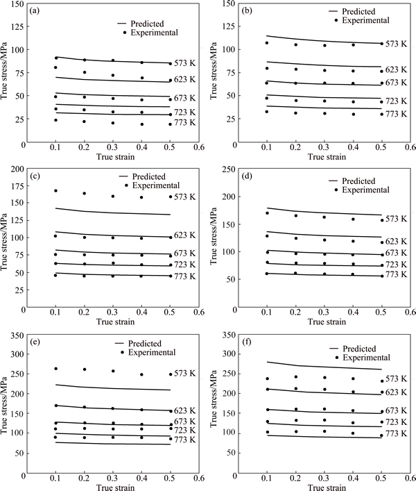
Fig. 9 Comparison between experimental and predicted flow stress values by modified Johnson-Cook model at strain rate of   0.001 s^-1 (a), 0.01 s^-1 (b), 0.1 s^-1 (c), 1 s^-1 (d), 10 s^-1 (e), 100 s^-1 (f)

Table 5 Constants for modified Johnson-Cook model

Multiplying each side by the natural logarithm,   Eq. (23) can be rearranged as follows:

                       (24)

Five values for m and I (σT*^β) for each temperature can be calculated from the slope of intercept respectively from the plot of  against  by performing a linear fit as shown in Fig. 10(a). Values for γ₁₁ and γ₁₂ can be calculated from the plot of m against T* as shown in Fig. 10(b) by performing a linear fit. Values for α and β can be calculated from the plot of I against T* by performing a first order power fit as shown in Fig. 10(b). At reference strain rate,   will yield 5 values represented at different temperatures. Hence, values for γ₂₁ and γ₂₂ can be calculated from the linear plot of  against T as shown in Fig. 10(c). will also yield 5 values represented at different temperatures. Values for γ₃₁ and γ₃₂ can be calculated from the plot of  against T by performing a linear fit as shown in Fig. 10(d). Table 6 shows the constants for the Maheshwari model. Using these constants, the   flow stress data are predicted under various processing conditions. Comparison between the experimental and predicted data by the Maheshwari model is shown in  Fig. 11.

Table 6 Constants for Maheshwari model

3.5 Khan-Liu model

The Khan-Liu model [23] is represented as follows:

        (25)

where σ is the flow stress, ε is the plastic strain,  is the dimensionless strain rate with  being the strain rate and  (1 s^-1) being the reference stain rate, T*=(T_melt-T)/(T_melt-T_ref) with T being the current temperature, T_ref (573 K) is the reference temperature, T_melt (911 K) is the melting temperature,  T_c (380 K) is the threshold temperature. Parameters A, B, C₁, C₃, n₀, K₁, m₁, m₂ and m₃ are all material constants. The material constant A can be determined from the yield stress at reference temperature and reference strain-rate. At reference temperature and zero plastic strain, Eq. (25) can be rearranged to

                              (26)

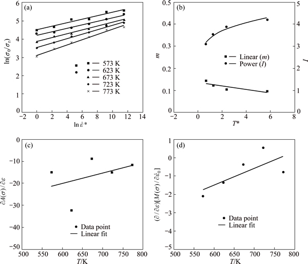
Fig. 10 Plot of ln(σ₀/σ_r) against (a), m and I against T* (b),  against T (c) and  against T (d)

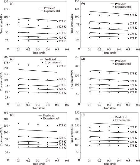
Fig. 11 Comparison between experimental and predicted flow stress values by Maheshwari model at strain rate of 0.001 s^-1 (a),  0.01 s^-1 (b), 0.1 s^-1 (c), 1 s^-1 (d), 10 s^-1 (e), 100 s^-1 (f)

Material constant C₁ can be calculated from the slope of ln(σ/A) against  by performing a linear fit as shown in Fig. 12(a). However, it is clear that this relationship would be more accurately represented by a power function fit. At reference strain rate and zero plastic strain, Eq. (25) can be rearranged to

                    (27)

Material constant m₂ can be determined from the slope of ln(σ_y/A) against   by performing a

linear fit as shown in Fig. 12(b). At reference strain rate, Eq. (25) can be rearranged to

  (28)

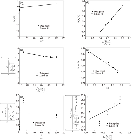
Fig. 12 Plots of ln(σ/A) against  (a),  ln(σ_y/A) against   (b),   against (c), ln(σ-A) against lnε (d),  against (e) and against  (f)

Material constant m₃ can be determined from the slope of  against  by

performing a linear fit as shown in Fig. 12(c). At reference strain rate and reference temperature, Eq. (25) can be rearranged to

ln(σ-A)=ln B+n₀ln ε                          (29)

Material constants n₀ and B can be determined from the slope and intercept respectively of ln(σ-A) against lnε by performing a linear fit as shown in Fig. 12(d). At reference temperature, Eq. (25) can be rearranged to

                (30)

Material constant C₃ can be determined from    the slope of  against  by

performing a linear fit as shown in Fig. 12(e). However, it is clear that a linear fit is not adequate for this relationship. According to KHAN and LIU [23], at fixed temperature (573 K), fixed strain (10%) and at fixed strain rates (0.001, 0.01 and 1 s^-1), K₁ can be calculated from

                   (31)

Furthermore, m₁ can be calculated from Eq. (32) by using stress data at elevated temperature and strain rates of 1 and 0.01 s^-1 as shown in Fig. 12(f). Table 7 shows the constants for the Khan-Liu model. Using these constants, the flow stress data are predicted under various processing conditions. Comparison between the experimental and predicted data by the Khan-Liu model is shown in Fig. 13.

  (32)

Table 7 Constants for Khan-Liu model

3.6 Trimble model

The Trimble model [27] can be represented as follows:

σ=Aεⁿexp(Bε+C)T*                           (33)

where σ is the flow stress, ε is the plastic strain,  is the strain rate, T*=(T-T_ref) with T being the current temperature and T_ref being the reference temperature, A and n represent the effect of work hardening, C is a material constant which incorporates the effect of temperature on flow stress, and B is the constant that defines the coupled effect of strain and temperature on flow stress. A reference temperature is used to avoid extrapolation of the flow stress to 0 K as data are not available at this temperature. The difference between the temperature of interest and the reference temperature is used to incorporate the effect of flow softening, with the reference temperature being the minimum temperature (573 K) of the test matrix for which prediction is required. To consider the effect of strain rate, material constants A, n, B and C are considered functions of strain rate which can be described as the third order polynomials as follows:

            (34)

The constants can be determined by multiplying each side of Eq. (33) by the natural logarithm:

ln σ=ln A+nln ε+(Bε+C)T*                     (35)

A linear plot of lnσ against T* as shown in      Fig. 14(a) yields five values for (Bε+C) represented by the slope (S) and five values of lnA+nlnε represented by the intercept (I) for each value of strain at one particular strain rate such that:

S=Bε+C                                    (36)

 

I=ln A+nln ε                                (37)

A linear plot of S against ε as shown in Fig. 14(b) will yield six values for B and C at different strain rates which can be calculated from the slope and intercept respectively. Similar, a linear plot of I against ln ε as shown in Fig. 14(c) will yield six values for A and n.   A third order polynomial plot of A, n, B and C againstas shown in Fig. 15 will yield values for all constants in Eq. (34). Table 8 shows the constants for the Trimble model. Using the optimised constants, the flow stress data are predicted under various processing conditions. Comparison between the experimental and predicted data using the Trimble model is shown in Fig. 16.

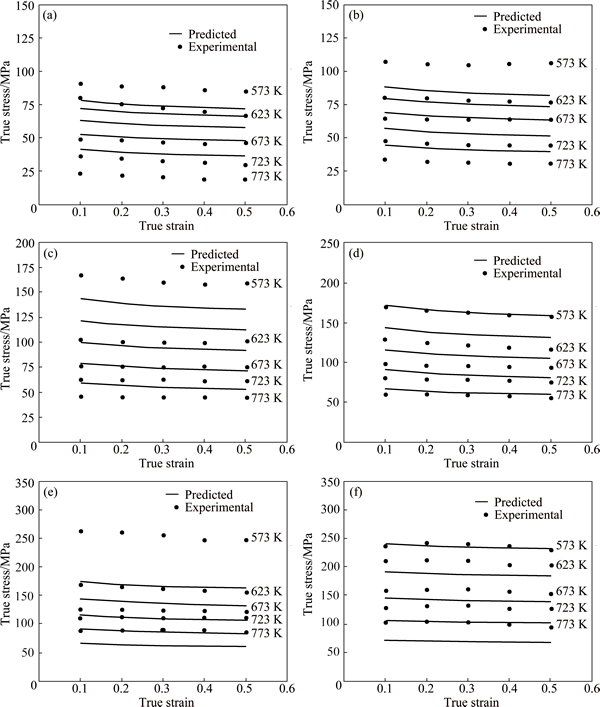
Fig. 13 Comparison between experimental and predicted flow stress values by Khan-Liu model at strain-rate of 0.001 s^-1 (a),    0.01 s^-1 (b), 0.1 s^-1 (c), 1 s^-1 (d), 10 s^-1 (e), 100 s^-1 (f)

Fig. 14 Plots of ln σ against T* at strain-rate of 1 s^-1 (a), S against ε (b), and I against ln ε (c)

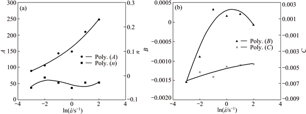
Fig. 15 Plot of A and n against  (a) and B and C against  (b)

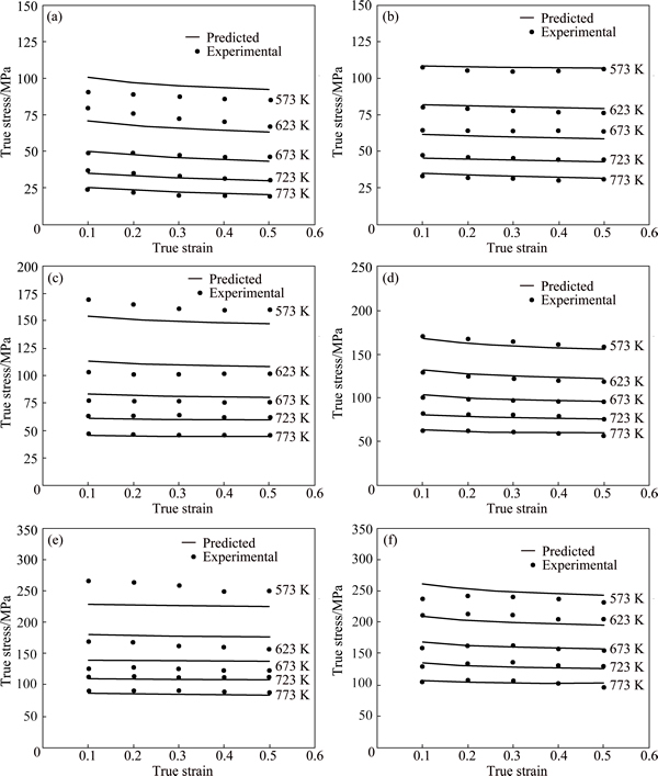
Fig. 16 Comparison between experimental and predicted flow stress values by Trimble model at strain rate of 0.001 s^-1 (a),      0.01 s^-1 (b), 0.1 s^-1 (c), 1 s^-1 (d), 10 s^-1 (e), 100 s^-1 (f)

Table 8 Constants for Trimble model

4 Discussion

In order to make a comparative analysis on the predictability of the models, the correlation coefficient  (R) and the average absolute relative error (AARE) were used to evaluate the deviation of the predicted flow stress. The correlation coefficient provides information on the strength of the linear relationship between the experimental and predicted values. It should be noted that a higher value of R may not necessarily indicate better performance due to the tendency of the model to be biased towards higher or lower values [29]. However, the average absolute relative error (AARE) is computedthrough a term by term comparison of the relative error and is therefore an unbiased statistical parameter for measuring the predictability of a model. The correlation coefficient and average absolute relative error (AARE) can be expressed as

                 (38)

                 (39)

where E_i is the experimental data and P_i is the predicted data, and are the mean experimental and predicted values respectively, and N is the total number of data employed in the analysis. Figure 17, Table 9 and Table 10 show the correlation between experimental and predicted flow stresses, the AARE at different strain rates and temperatures, and the overall AARE and correlation coefficient for the six models investigated respectively. The recently developed Trimble model recorded the highest correlation coefficient (R=0.99) and the lowest AARE (4.6%) across all models investigated and hence is the most suitable for predicting the hot deformational behaviour of 2024Al-T3 alloy across the processing domain investigated during this analysis. The empirical formulation of the model ensures that the coupled effects of strain, strain rate and temperature are encapsulated when predicting flow stress and constants are calculated over the entire processing domain.

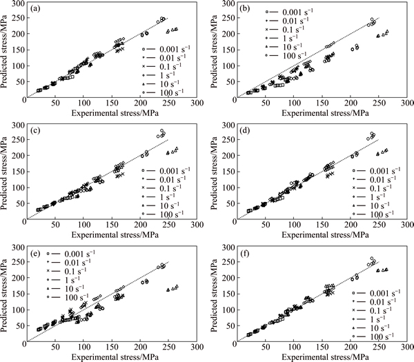
Fig. 17 Correlation between experimental and predicted flow stress values for different constitutive models: (a) Arrhenius-type compensation model; (b) Johnson-Cook model; (c) Modified Johnson-Cook model; (d) Maheshwari model; (e) Khan-Liu model;  (f) Trimble model

Table 9 AARE at different strain-rate and temperature for different constitutive models

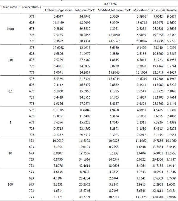
Table 10 Total AARE and correlation coefficient for different constitutive models

In comparison, some models make assumption to calculate constants within specific processing ranges which reduce prediction capability. For example, when determining the constants of the Johnson-Cook model, constants A, B and n are calculated at the reference strain (1 s^-1) and reference temperature (573 K). As a result, a low AARE of 0.4984% is recorded in this condition compared with an average AARE of 25.09%. Constant C is calculated at reference temperature and AARE values are on average less at this temperature compared with others (15.78% at 573 K, 23.69% at 623 K, 24.13% at 673 K, 29.32% at 723 K, 32.54% at 773 K). Hence, four of the five constants of this model are calculated within a narrow processing window of reference temperature and strain rate.

Similarly, constants P, Q and n of the modified Johnson-Cook model are all calculated at the reference strain rate (0.001 s^-1) and reference temperature (573 K). As a result, a low AARE of 0.566% is recorded in this condition compared with an average of 7.933%. Constant r is calculated at reference temperature and AARE values are on average less at this temperature compared with others (3.42% at 573 K, 4.73% at 623 K, 6.59% at 673 K, 9.23% at 723 K, 15.68% at 773 K). Hence, four of the six constants of this model are calculated within a narrow processing window.

Also, constants A, B and n₀ of the Khan-Liu model are all calculated at the reference strain rate (1 s^-1) and reference temperature (573 K) and a low AARE of 4.54% is recorded in this condition compared with an average value of 19.31%. Constants C₁ and C₂ are calculated at reference temperature and constants m₁ and m₃ are calculated at reference strain rate. Hence, seven of the nine constants of this model are calculated within a narrow processing window.

A number of minor assumptions reduce the prediction capability of the Arrhenius-type model. For example, it is assumed that there is a constant linear relationship between σ against  at all temperatures. However, this is not the case as shown in Fig. 3(b). It is clear that the slope decreases with increasing temperature which must be accounted for. Further constant linear assumptions can be observed in Fig. 3(a). Similarly, MAHESHWARI assumed constant linear relationships in Figs. 10(c) and (d) when this is not the clear case.

Table 11 shows the prediction capability of different models using constants from literature (Table 1) over the processing domain investigated during this analysis. As expected, values of AARE and correlation coefficient are significantly higher and lower respectively compared with those in Table 10. This can be attributed to a variation of the processing domain investigated to determine these constants, material composition and heat treatment compared with this analysis.

Table 11 Prediction capability using constants from literature

5 Conclusions

Isothermal hot compression tests were conducted on a Gleeble-3800 mechanical simulator over a wide processing range of strain (0.1-0.5), temperatures (573-773 K) and strain rate (0.001-100 s^-1) to predict the hot deformational behaviour of 2024Al-T3 alloy.  Statistical parameters such as correlation coefficient and average absolute relative error were used to determine the prediction capability of various constitutive models for 2024Al alloys and a recently developed model. The Trimble model recorded the lowest AARE (4.6%) and the highest correlation coefficient (R=0.99) compared with other models. Hence, the Trimble model is the most suitable for predicting the hot deformational flow stress behaviour of 2024Al-T3 alloy across the processing range investigated during this analysis.

References

[1] LIN Y C, XIA Yu-Chi, CHEN Ming-Song, JIANG Yu-Qiang, LI Lei-Ting. Modelling the creep behaviour of 2024-T3 Al alloy [J]. Computational Material Science, 2013, 67: 243-248.

[2] TRIMBLE D, O’DONNELL G E, MONAGHAN J. Characterisation of tool shape and rotational speed for increased speed during friction stir welding of AA2024-T3 [J]. Journal of Manufacturing Processes, 2015, 17: 141-150.

[3] MAHMOODKHANI Y, WELLS M A, PARSON N, POOLE W J. Numerical modelling of the material flow during extrusion of aluminium alloys and transverse weld formation [J]. Journal of Materials Processing Technology, 2014, 214: 688-700.

[4] SCHINDLER S, ZIMMERMANN M, AURICH J C, STEINMANN P. Thermo-elastic deformations of the workpiece when dry turning aluminium alloys—A finite element model to predict thermal effects in the workpiece [J]. CIRP Journal of Manufacturing Science and Technology, 2014, 7: 233-245.

[5] PATURI U M R, NARALA S K R, PUNDIR R S. Constitutive flow stress formulation, model validation and FE cutting simulation for AA7075-T6 aluminium alloy [J]. Material Science and Engineering A, 2014, 605: 146-185.

[6] TRIMBLE D, MONAGHAN J, O’DONNELL G E. Force generation during friction stir welding of AA2024-T3 [J]. CIRP Annals- Manufacturing Technology, 2012, 61: 9-12.

[7] SAMANTARAY D, MANDAL S, BHADURI A K. Constitutive analysis to predict high temperature flow stress in modified 9Cr-1Mo (P91) steel [J]. Materials and Design, 2010, 31: 981-984.

[8] MANDAL S, RAKESH V, SIVAPRASAD P V. Constitutive equations to predict high temperature flow stress in Ti-modified austenitic stainless steels [J]. Material Science and Engineering A, 2009, 500: 114-121.

[9] SUNG J H, KIM J H, WAGONER R H. A plastic constitutive equation incorporating strain, strain rate and temperature [J]. International Journal of Plasticity, 2010, 26: 1746-1771.

[10] ZENER C, HOLLOMON H. Effect of strain rate upon plastic flow of steel [J]. Journal of Applied Physics, 1944, 15: 22-32.

[11] SELLARS C M, TEGART W J Mc G. Hot workability [J]. International Materials Reviews, 1972, 17: 1-24.

[12] SHEPPARD T, JACKSON A. Constitutive equations for use in prediction of flown stress during extrusion of aluminium alloys [J]. Material Science and Technology, 1997, 13: 203-209.

[13] CEPEDA-JIMENEZ C M, RUANO O A, CARSI M, CARRENO F. Study of hot deformation of an Al-Cu-Mg alloy using processing maps and microstructural characterization [J]. Material Science and Engineering A, 2012, 552: 530-539.

[14] HAO Shi-ming, XIE Jing-pei, WANG Ai-qui, WANG Wen-yan, LI Ji-wen, SUN Hao-liang. Hot deformation behaviour of 35%SiC_p/2024Al metal matrix composites [J]. Transactions of Nonferrous Metals Society of China, 2014, 24(8): 2468-2474.

[15] LIN Y C, CHEN M S, ZHONG J. Constitutive modelling for elevated temperature flow behaviour of 42CrMO steel [J]. Computational Material Science, 2008, 42: 470-477.

[16] JOHNSON G R, COOK W H. A constitutive model and data for metals subjected to large strains, high strain rates and high temperatures [C]//Proceedings of the 7th International Symposium on Ballistics. The Hague, The Netherlands, 1983: 541-547.

[17] LESUER D R. Experimental investigations of material models for Ti-6Al-4V titanium and 2024-T3 aluminium [R]. DOT/FAA/AR-00/25, US Department of Transport, Federal Aviation Administration, 2000.

[18] SEIDT J D, GILAT A. Plastic deformation of 2024-T351 aluminium plate over a wide range of loading conditions [J]. International Journal of Solids and Structures, 2013, 50: 1781-1790.

[19] AMIR H A S, MADHAVAN V, BEHNAM B. Extension of oxley’s analysis of machining to use different material models [J]. Journal of Manufacturing Science and Engineering, 2003, 125: 656-666.

[20] OXLY P L B. The mechanics of machining: An analytical approach to assessing machinability [M]. Chishester, England: Ellis Horwood, New York: Halsted Press, 1989.

[21] MAHESHWARI A K, PATHAK K K, RAMAKRISHNA N, NARAYAN S P. Modified Johnson-Cook material flow model for hot deformation processing [J]. Journal of Material Science, 2010, 45: 859-864.

[22] MAHESHWARI A K. Prediction of flow stress for hot deformation processing [J]. Computational Materials Science, 2013, 69: 350-358.

[23] KHAN A S, LIU H. Variable strain rate sensitivity in an aluminium alloy: Response and constitutive modeling [J]. International Journal of Plasticity, 2012, 36: 1-14.

[24] LIN Y C, DING Yi, CHEN Ming-Song, DENG Jiao. A new phenomenological constitutive model for hot tensile deformation behaviours of a typical Al-Cu-Mg alloy [J]. Materials and Design, 2013, 52: 118-127.

[25] LIN Y C, LI L T, JIANG Y Q. A phenomenological constitutive model for describing thermos-viscoplastic behaviour of Al-Zn-Mg-Cu alloy under hot working condition [J]. Experimental Mechanics, 2012, 52: 993-1002.

[26] LIN Y C, LI L T, FU Y X, JIANG Y Q. Hot compressive deformation behaviour of 7075 Al alloy under elevated temperature [J]. Journal of Materials Science, 2012, 47: 1306-1318.

[27] TRIMBLE D, O’DONNELL G E. Constitutive modelling for elevated temperature flow behaviour of AA7075 [J]. Materials and Design, 2015, 76: 150-168.

[28] ASTM E209. Standard practice for compression tests of metallic materials at elevated temperatures with conventional or rapid heating rates and strain rates [S]. 2010.

[29] SAMANTARAY D, MANDAL S, BHADURI A K. A comparative study on Johnson-Cook, modified Zerilli-Armstrong and Arrhenius-type constitutive models to predict elevated temperature flow behaviour in modified 9Cr-1Mo steel [J]. Computational Materials Science, 2009, 47: 568-576.

Al2024-T3合金热变形加工工艺的流变应力预测

D. TRIMBLE, G. E. O’DONNELL

Department of Mechanical & Manufacturing Engineering, Trinity College Dublin, College Green, Dublin 2, Ireland

摘  要：为了预测Al2024-T3合金热变形加工工艺的流变应力行为，在应变速率(0.001~100 s^-1)、应变(0.1~0.5)和温度(573~773 K)条件下，进行了等温压缩试验。采用统计参数，如平均相对误差绝对值(AARE)和相关系数(R)评估了Al2024合金不同的本构模型和最新构建的本构模型的预测能力。与其他的模型相比，最新构建的模型能得到最低的AARE(4.6%)和最高的相关系数(0.99)。因此，与其他模型相比，该模型能更精确地描述Al2027-T3合金的变形行为。

关键词：等温压缩；2024铝合金；本构模型；流变应力

 (Edited by Xiang-qun LI)

Corresponding author: D. TRIMBLE; Tel: +353-1-8964856; Fax: +353-1-6795554; E-mail: trimbled@tcd.ie

DOI: 10.1016/S1003-6326(16)64194-8