J. Cent. South Univ. Technol. (2011) 18: 1654-1661

DOI: 10.1007/s11771-011-0885-1

Strain analysis of buried steel pipelines across strike-slip faults

WANG Bin(王滨), LI Xin(李昕), ZHOU Jing(周晶)

State Key Laboratory of Coastal and Offshore Engineering, Dalian University of Technology, Dalian 116024, China

? Central South University Press and Springer-Verlag Berlin Heidelberg 2011

Abstract: Existing analytical methods of buried steel pipelines subjected to active strike-slip faults depended on a number of simplifications. To study the failure mechanism more accurately, a refined strain analytical methodology was proposed, taking the nonlinear characteristics of soil-pipeline interaction and pipe steel into account. Based on the elastic-beam and beam-on-elastic- foundation theories, the position of pipe potential destruction and the strain and deformation distributions along the pipeline were derived. Compared with existing analytical methods and three-dimensional nonlinear finite element analysis, the maximum axial total strains of pipe from the analytical methodology presented are in good agreement with the finite element results at small and intermediate fault movements and become gradually more conservative at large fault displacements. The position of pipe potential failure and the deformation distribution along the pipeline are fairly consistent with the finite element results.

Key words: strike-slip fault; buried pipeline; nonlinear pipe-soil interaction; analytical formula; strain analysis

1 Introduction

Large differential ground movements from an active fault probably represent one of the most severe earthquake effects on a buried pipeline. The axial and bending strains induced to the pipeline by fault movements may become fairly large and result in  rupture, which can cause catastrophic disruption of important urban infrastructures, even lead to irrecoverable ecological disasters.

In recent years, numerical analysis based on finite element methods [1-4] has been available for solving the problem. Nevertheless, the non-linear behaviors of pipeline steel, the soil and pipeline interaction and the large displacements make such analysis rather time- consuming, which provides background for the use of simplified analytical methods, at least for preliminary design and verification purposes.

An analytical method proposed by NEWMARK and HALL [5] adopted a small displacement model with static soil pressure and static friction force to study the effects of fault displacements on buried pipelines. Passive soil resistance was not taken account.

Later, KENNEDY et al [6] extended NEWMARK and HALL’s procedure by considering pipe-soil interaction in the transverse direction. Based on a circle arc model, a pipeline was modeled as a cable with tension stiffness but no flexural stiffness. This assumption restricts the application of the analytical method to the case of large fault movements in projection to the pipe axial direction.

To improve KENNEDY et al’s study, WANG and YEH [7] took the pipe flexural stiffness into account. The adopted model was based on the partitioning of pipeline into four segments: two segments in the high curvature zone on both sides of the fault trace were assumed to deform as circular arcs, while another two segments outside this zone were treated as beams on elastic foundations. Although it is clearly advanced, the model has some pitfalls, specially:

1) The unfavorable contribution of axial force to the flexural stiffness is overlooked.

2) The continuous condition of the shear force at the conjunction of arc with its neighboring beam on elastic foundation is ignored.

3) The position of pipe potential damage is not necessarily determined at the two ends of the high-curvature zone on each side of the fault trace as the method assumes, but within the zone, it is closer to the intersection with the fault trace.

More recent study by KARAMITROS et al [8] introduced a number of refinements to the above mentioned method. A pipeline was also partitioned into four segments, whereas the elastic-beam model was adopted in the high-curvature zone on both sides of fault trace, instead of the circular-arc model from WANG and YEH’s method. The continuous condition of the shear force at the conjunction of elastic beam with its neighboring beam on elastic foundation was considered, as well as the actual distribution of stresses on the pipeline cross-section. The analytical method also have some shortcomings:

1) A combination of bending strain based on the elastic beam theory and bending strain induced by second-order effects is introduced to take into account of the effect of axial force on the flexural stiffness. Compared with the numerical results, the adopted combination form provides a rather good approximation to real strains but lacks physical meaning.

2) Due to ignoring the pipe-soil friction force in the high-curvature zone, the position of pipe potential damage is erroneously defined at the maximum bending-moment cross section. No numerical validations of the pipe damage position are given.

3) The secant modulus of the bilinear stress-strain relationship for pipe steel is employed as the elastic modulus of the elastic-beam segment. The secant modulus is a constant when the pipe stress is less than or equal to the yielding stress. Thus, if the initial value of the elastic modulus of the elastic-beam segment is selected unsuitably, the iteration will not be converged. How to obtain the proper initial value is not described.

4) The nonlinearity of pipe-soil interaction is disregarded. To study the failure mechanism of buried pipelines due to faulting more accurately, the effects of nonlinear pipe-soil interaction have to be considered [9-12].

Considering the soil-pipeline nonlinear interaction referred to American Lifeline Alliance (ALA) [13], a refined strain analytical methodology for buried pipelines across strike-slip faults was proposed in this work. Some modifications of KARAMITROS’ method were made, namely,

1) The elastic modulus of pipe in the high-curvature zone was obtained according to the maximum axial total stain of pipe. Hence, the effect of axial force on the flexural stiffness was considered, and the physical meaning was clear.

2) A Ramberg-Osgood model was introduced to simulate the elasto-plasticity property of pipe steel. Since the adopted tangent modulus of the model was monotonically decreased with increasing the engineering stresses, the iteration procedure was assured to converge definitely.

3) The exact position of pipe potential destruction and the distributions of strain and deformation along the pipeline were derived and validated by the comparison with three-dimensional nonlinear finite element analysis.

2 Constitutive models

2.1 Ramberg-Osgood stress-strain relationship of pipe steel

To avoid judging pipe material yielding conditions used in KARAMITROS’ method, a Ramberg-Osgood model is selected to simulate the elasto-plasticity property of pipe steel. The expression of stress-strain relationship is

                                                    (1)

                                   (2)

where ; ; ;  and  are

the engineering strain and stress, respectively; E₀ is the initial elastic modulus; σ_y is the yielding stress of pipe steel; n and r are the Ramberg-Osgood parameters; E_tag,x is the tangent elastic modulus. Since the adopted tangent modulus of the model is monotonically decreased with increasing the engineering stresses, the subsequent nonlinear iteration procedure can converge definitely in each iterative step.

2.2 Pipe-soil nonlinear interaction

The pipe-soil nonlinear interactions in the axial and lateral directions herein are simulated as the elastic perfectly-plastic soil springs recommended by American Lifeline Alliance (ALA) [13].

3 Analytical methodology outline

3.1 Basic assumptions

1) A strike-slip fault is taken as an inclined plane, i.e. with null width of rupture zone.

2) The initial pipeline stresses due to soil overburden and pipeline laid are ignored.

3) Pipeline and soil inertia effects are not taken into account.

4) Local buckling and section deformation effects are neglected.

3.2 Description of problem

Based on the concept originally introduced by WANG and YEH [7], the pipeline is partitioned into four segments, as shown in Fig.1. Only half of the pipe structure (segment A′B) is analyzed due to the anti- symmetrical deformation of buried pipeline under a strike-slip fault. In Fig.1, point B is the intersection of the pipeline axis with the fault trace, where the bending moment equals zero, while points A and C are the closest points of the pipeline axis from point B with zero lateral pipe-soil relative displacement. Points A′ and C′ are at a distance from A and C which is sufficient for the attenuation of lateral displacements.

The fault movement is defined in a Cartesian coordinate system, where x-axis is parallel to the longitudinal axis of the undeformed pipeline, y-axis is perpendicular to x in the horizontal plane, and β is the crossing angle of the fault trace and x-axis (Fig.1). In its present form, the proposed method applies the crossing angles of 0<β<90°, which results in the pipeline elongation. The fault displacement shown in Fig.1 is defined as Δ_f. The intersection B moves one-half of Δ_f. ΔX and ΔY are respectively the axial and lateral components of fault displacements in one side of fault. L_A is the length of the pipe-soil large deformation segment in one side of fault. f_L and q(x) are the axial and lateral soil spring forces per unit length of pipeline, respectively.

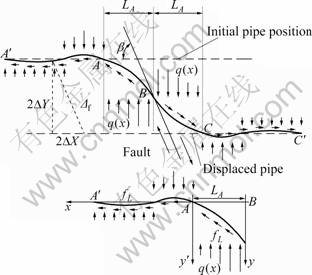
Fig.1 Partitioning of buried pipelines under strike-slip faults

3.3 Definitions of terms

Some terms used in this work are defined as follows:

1) The geometrical elongation of pipeline is the pipe deformation obtained from the geometrical compatibility conditions subjected to fault movements.

2) The physical elongation of pipeline is the pipe deformation resulted from the integration of axial strain along the unanchored length of pipe.

3) The unanchored length of pipeline is the one where the relative slippage occurs between the pipe and the surrounding soil. The unanchored length certainly increases with increasing the fault movements.

4 Solution algorithm

4.1 Axial response analysis of pipeline

The geometrical elongation of pipe ΔL_g is

                            (3)

where L is the unanchored length. For the sake of simplicity, the geometrical elongation provoked by the lateral fault displacement component ΔY may be neglected, as ΔY ²/2L is much less than ΔX.

The physical elongation of pipe, ΔL_p, is given by

                                                              (4)

where ε_a is the axial strain of the unanchored segment.

According to the yielding states of axial soil springs, two cases are classified.

4.1.1 Elastic case for axial soil springs

In Fig.2, point O is the closest point of the pipeline axis from the intersection B with zero axial pipe-soil relative displacement, L is the pipe unanchored length, point P is the hypothetical point where the axial soil spring just yields, and L₀ is the pipe maximum length of the non-yielding segment of axial soil springs. The pipe elongation of segment OP is u₀ equal to the yielding displacement of axial soil spring, i.e. the pipe-soil axial relative displacement of point P is u₀. Since the axial soil springs are still elastic along the pipeline, the pipe elongation of segment L is less than or equal to the yielding displacement of axial soil spring, i.e. ?X≤u₀, L≤L₀.

Fig.2 Pipe axial elongation of unanchored segment without yielding of axial soil spring

The axial soil spring force per unit length of pipe is assumed to be linear along segment L₀, thus, it can be expressed as

                                                (5)

where f_s is the maximum axial soil spring force per unit length of pipe.

Then, the axial stress at the intersection of the pipeline with the fault trace σ_a,B is:

                                          (6)

where A_s is the area of pipeline cross-section, A_s=(π/4)× (D²-d²)=πt(D-t), t is the wall thickness of pipe, D and d are the pipe outside and inner diameters, respectively.

Since the physical elongation of segment L₀ equals u₀, L₀ is obtained by

                           (7)

As the physical elongation of pipeline equals the geometrical one, L is determined by

                   (8)

4.1.2 Yielding case for axial soil springs

For the yielding of the axial soil springs, the pipe elongation of segment L is larger than the yielding displacement of axial soil spring, i.e. ?X>u₀, L>L₀. To take the axial pipe-soil nonlinear interaction into account, the unanchored pipeline is divided into two parts, as shown in Fig.3, namely, L₀ and L₁. The axial soil springs of segment L₀ keep elastic, while the axial soil springs of segment L₁ yield totally. Point E is the critical point where the axial soil spring just yields. The physical elongation of segment L₀ equals the yielding displacement of axial soil spring u₀.

Fig.3 Pipe axial elongation of unanchored segment with yielding of axial soil spring

The axial stress σ_a,E at the conjunction point of segment L₀ and L₁ is given by

                                          (9)

where L₀ is obtained by solving Eq.(7).

The axial soil springs completely yield in the range of L₀≤x≤L, then, the unanchored length L can be calculated as

                                                     (10)

The pipe physical elongation ?L₁ of segment L₀≤x≤ L is

                           (11)

where ; .

Since the pipe geometrical elongation equals the pipe physical elongation, there is

                                                            (12)

Substituting Eq.(11) into Eq.(12), the axial stress σ_a,B at the intersection of the pipeline with the fault trace is obtained. Then, the pipe unanchored length L is calculated from Eq.(10).

4.2 Lateral response analysis of pipeline

4.2.1 Segment AA′ analysis

Based on the beam-on-elastic-foundation theory and the assumption that the elastic modulus of segment AA′ is the initial elastic modulus for pipe steel due to the comparatively small deformation, the differential equilibrium equation of segment AA′ on the basis of the xAy′ coordinate system shown in Fig.1 is taken as

                                                 (13)

where y is the lateral pipe-soil relative displacement; k is the constant of the lateral soil spring; I is the moment of

inertia of the pipeline cross-section,

Introducing the boundary conditions, y→0 at x→∞ and y=0 at x=0, and transforming xAy′ coordinate system into xBy one in Fig.1, Eq.(13) is solved by

              (14)

where , and C₄ is a unknown constant.

4.2.2 Segment AB analysis

Based on the yielding states of lateral soil springs, two cases are divided as follows.

1) Elastic case for lateral soil springs

In Fig.4,  in which Δ_P is the

yielding displacement of lateral soil spring. Based on the beam-on-elastic-foundation theory as well, the expression for y is obtained in xBy coordinate system:

         (15)

where D₁, D₂, D₃, and D₄ are unknown constants, λ_AB=

 and E_AB is the elastic modulus of segment

AB, which is the tangent elastic modulus of Ramberg- Osgood model for pipe steel corresponding to the maximum axial total stain of segment AB.

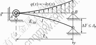
Fig.4 Sketch of pipe-soil large deformation segment AB without yielding of lateral soil spring

Therefore, the pipe-soil lateral relative displacement is taken as

             (16)

From the boundary conditions and compatibility requirements, the following equations are found:

                                         (17)

2) Yielding case for lateral soil springs

In Fig.5,the lateral soil spring

at point D just yields. L_D is the pipe maximum length of the yielding segment of lateral soil springs, and q_u is the maximum lateral soil spring force per unit length of pipe. Using the elastic-beam theory, the differential equilibrium equation of segment DB in xBy coordinate system is taken as

                                                       (18)

where E_DB is the elastic modulus of segment DB, which is the tangent elastic modulus of Ramberg-Osgood model for pipe steel corresponding to the maximum axial total stain of segment DB. The general homogeneous solution to Eq.(18) is

        (19)

where G₁, G₂, G₃, and G₄ are unknown constants.

Fig.5 Sketch of pipe-soil large deformation segment AB with yielding of lateral soil spring

The beam-on-elastic-foundation theory is adopted in the analysis of segment AD, where the lateral soil springs are elastic. In combination with Eq.(14), the pipe-soil lateral relative displacement is given by

      (20)

where H₁, H₂, H₃ and H₄ are unknown constants; λ_AD=

 E_AD is the elastic modulus of segment AD,

which is the tangent elastic modulus of Ramberg-Osgood model for pipe steel corresponding to the maximum axial total stain of segment AD.

Based on the boundary conditions and compatibility requirements, the following equations are obtained:

                                     (21)

Therefore, the pipe lateral displacement Δ_pipeline is

                                                       (22)

where Δ_soil is the soil lateral displacement.

4.3 Determination of axial total strain

As mentioned previously, the axial stain of the unanchored pipe is obtained by introducing the corresponding axial stress into Eq.(1), and the bending stain of unanchored pipe is solved by the corresponding

curvature, i.e.By summing up the bending

and axial strains, the axial total strain ε_t,x of arbitrary position along the unanchored pipeline is expressed as

                       (23)

where B_a,x is related to the yielding states of the axial soil springs. For the non-yielding of the axial soil springs, measured from the intersection B, B_a,x can be expressed as

                       (24)

For the yielding of the axial soil springs, according to post-earthquake surveys and finite element analysis, the axial soil springs in the pipe-soil large deformation segment AB will yield whether the lateral soil springs in the segment AB yield or not, i.e. L₁>L_A always exists, measured from the intersection B. In this case, B_a,x can be expressed as

                  (25)

An extreme value function is expressed by taking derivative of ε_t,x with respect to x in Eq.(23):

      (26)

The maximum axial total strain position x_max in the pipe-soil large deformation segment is obtained by solving Eq.(26). Introducing x_max into Eqs.(23), (1), and (2), the elastic modulus in the pipe-soil large deformation segment can be obtained.

Based on the yielding states of axial and lateral soil springs, corresponding equations are selected from Eq.(1), (2), (17), (21), (23), (24), (25) and (26). Solving the equations, the abovementioned unknown numbers, D₁-D₄, G₁-G₄, H₁-H₄, C₄, E_AB, E_AD, E_DB, λ_AB, λ_AD, L_A and L_D, can be obtained. Introducing the results into Eq.(16), (20) and (23), the analytical formulas of strain and deformation along the pipeline can be obtained, as well as the pipe maximum axial total strain and the pipe potential failure position.

4.44.4 Analysis procedure

Four steps are carried out in the analysis:

1) The axial stresses at the intersection and the pipe unanchored length are determined by equalizing the geometrical and physical elongations of pipeline.

2) Applying the beam-on-elastic-foundation and elastic-beam theories, the expressions of lateral pipe-soil relative displacement are obtained.

3) Combined with the axial and lateral analysis of pipeline, the expressions of axial total strain can be taken.

4) Based on the pipe steel constitutive model, the boundary conditions and the compatibility requirements, the analytical formulas of strain and deformation along the pipeline can be solved by iterative methods.

55 Validation of proposed methodology

To validate the proposed methodology, analytical predictions were compared with the results from the available analytical methods and three-dimensional nonlinear finite element analyses using ADINA [14]. For this purpose, a typical buried steel pipeline was selected, featuring the outside diameter D=0.4 m, the wall thickness t=9.5×10^{-3 m, and the total length L}_FEM= 1.2×10³ m.

A pipe-shell element [14] that allowed the cross-section to ovalize and warp was employed to establish the pipeline finite element (FE) model. The pipe-shell element length was 1 m, and each element had 4 nodes.

To simulate soil-pipe interaction, two ends of each pipe-shell element were connected to axial, lateral and vertical soil springs using elastic perfectly-plastic spring elements. The properties of soil springs listed in Table 1 were calculated according to the ALA guidelines [13], assuming that the pipeline centerline was buried under 1.04 m of loose sand with internal friction angle of 33° and unit weight of 16.7 kN/m³. The coating dependent factor relating the internal friction angle of the soil to the friction angle at the soil-pipe interface, f, was 0.7. The strike-slip fault movement, Δ_f=10 m, was statically applied with the crossing angle β=70°.

Table 1 Soil spring properties in numerical analysis

The API SPEC 5L X60 pipeline steel was characterized by a Ramberg-Osgood stress-strain curve with the initial elastic modulus E₀=2.1×10¹¹ Pa, yielding stress σ_y=413 MPa, n=10 and r=12 [15]. Newmark’s method adopted the tri-linear stress-strain curve of pipe steel with the yielding stress σ₁=465 MPa, yielding strain ε₁=2.4×10^-3, failure stress σ₂=516 MPa and failure strain ε₂=4×10^-2 [16].

The results of the numerical analysis and analytical predictions from Newmark’s method, Kennedy’s method and proposed method are shown in Figs.6-8.

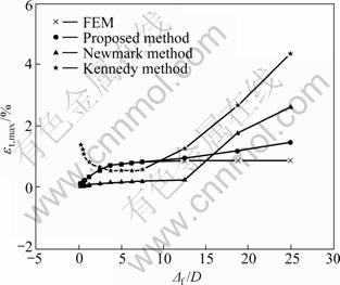
Fig.6 Effects of fault displacements on pipe maximum axial total strain

The variation of pipe maximum axial total strains with fault movements is shown in Fig.6. It can be seen that the analytical predictions from the proposed method are in good agreement with the numerical results of three-dimensional nonlinear FE analysis in the range of Δ_f≤10D. The deviations between analytical results proposed herein and numerical ones gradually increase in the range of Δ_f≥12.5D. The reason is that the initial elastic modulus E₀ of pipe steel is still selected as the elastic modulus of segment AA′ under larger fault movements, which results in the elastic modulus of the segment gradually larger than the actual one. Furthermore, the effect of geometric stiffness on pipeline response is not taken account in the proposed method. Thus, the maximum axial total strains from the proposed method are more conservative than those from FE method under large fault movements. In fact, the range Δ_f≤12.5D is rarely exceeded. Accordingly, the proposed method is suitable for engineering applications.

Two different values of fault movement Δ_f=10D and Δ_f=25D are selected for the comparative analysis. Figures 7(a) and (b) display the distributions of pipe axial total strain under the two fault movements, respectively. The positions of pipe maximum axial total strains from both the proposed analytical method and the numerical method are close to intersection B and fairly consistent. Thus, the method presented herein can accurately predict the potential damage position of buried steel pipeline under a strike-slip fault. Moreover, Fig.7 also displays that the pipe axial total strain calculated by the proposed method becomes gradually more conservative with increasing the fault displacements. Due to taking large-displacement effect, local buckling and section deformation into account in FE analysis, which actually exist near the position of pipe maximum axial total strain, the sudden decrease occurs with increasing the distances from the intersection after reaching the peak strain; while the proposed method does not takes account of the above factors, thereby, the analytical results show gradual decrease with increasing the distances from the intersection. Hence, the closed- shell-moment theories should be adopted for more accurate results.

Fig.7 Pipe axial total strain along pipeline: (a) Δ_f=10D; (b) Δ_f= 25D

Figures 8(a) and (b) show the distributions of pipe-soil lateral relative displacement under the fault movements Δ_f=10D and Δ_f=25D, respectively. The results from the proposed method herein are very close to the FEM ones, which proves the beam-on-elastic- foundation and elastic-beam models are suitable to simulate the lateral deformation of buried steel pipeline subjected to strike-slip faults.

Fig.8 Pipe-soil lateral relative displacement along pipeline:  (a) Δ_f=10D; (b) Δ_f=25D

66 Conclusions

1) Considering the nonlinearity of soil-pipeline interaction, a refined strain analytical methodology of buried steel pipelines subjected to active strike-slip faults is proposed. The effect of axial force on flexural stiffness is taken into account with the definitely physical meaning. The iteration procedure can converge definitely due to introducing the Ramberg-Osgood constitutive model of pipe steel. The position of pipe potential damage is derived, as well as the strain and deformation distributions along the pipeline.

2) The pipe maximum axial total strain from the analytical methodology presented are in good agreement with that from the FE analysis in the range of Δ_f≤10D and become gradually more conservative under large fault displacements Δ_f≥12.5D. In practice, the range Δ_f≤12.5D is rarely exceeded, thus, the proposed method is suitable for engineering applications.

3) The exact position of pipe potential failure, which is close to the intersection of pipeline axis with the fault trace, can be predicted by the analytical method.

4) The pipe-soil lateral relative displacements calculated by the analytical method herein are fairly consistent with the FE analysis results. Thus, the beam-on-elastic-foundation and elastic-beam models can simulate the lateral deformation of buried steel pipeline subjected to a strike-slip fault very well.

5) A buried pipeline is a thin-wall and hollow cylindrical shell, however, beam models and small deformation theories adopted in the proposed methodology do not take account of local buckling and section deformation of a pipeline. Therefore, it is of necessity to apply closed-shell-moment theories for more accurate analysis. Meanwhile, the interaction between bending and axial strains needs to be studied further.

References

[1] GU Xiao-ting, ZHANG Hong. Research on aseismatic measures of gas pipeline crossing a fault for strain-based design [C]// Pressure Vessels and Piping Conference 2009. Prague, Czech Republic: American Society of Mechanical Engineers, 2010: 571-580.

[2] JIAO Zhong-liang, SHUAI Jian, HAN Ke-jiang. Response analysis of buried pipeline subjected to fault movements [C]// International Conference on Pipelines and Trenchless Technology 2009: Advances and Experiences with Pipelines and Trenchless Technology for Water, Sewer, Gas, and Oil Applications. Shanghai, China: American Society of Civil Engineers, 2009: 1212-1218.

[3] LIU Ming, WANG Yong-yi, YU Zhi-feng. Response of pipelines under fault crossing [C]// Proceedings of the International Offshore and Polar Engineering Conference. Vancouver, BC, Canada: International Society of Offshore and Polar Engineers, 2008: 162-165.

[4] ZHU Qing-jie, CHEN Yan-hua, LIU Ting-quan, DAI Zhao-li. Finite element analysis of fluid-structure interaction in buried liquid-conveying pipeline [J]. Journal of Central South University of Technology, 2008, 15(Suppl. 1): 307-310.

[5] NEWMARK N M, HALL W J. Pipeline design to resist large fault displacement [C]// Proceedings of US Conference on Earthquake Engineering. Ann Arbor, Michigan: Earthquake Engineering Research Institute, 1975: 416-425.

[6] KENNEDY R P, CHOW A W, WILLIAMSON R A. Fault movement effects on buried oil pipeline [J]. Transportation Engineering Journal, 1977: 617-633.

[7] WANG L R L, YEH Y H. A refined seismic analysis and design of buried pipeline for fault movement [J]. Earthquake Engineering and Structural Dynamics, 1985, 13: 75-96.

[8] KARAMITROS D K, BOUCKOVALAS G D, KOURETZIS G P. Stress analysis of buried steel pipelines at strike-slip fault crossings [J]. Soil Dynamics and Earthquake Engineering, 2006, 27: 200-211.

[9] HA D, ABDOUN T H, O'ROURKE M J. Soil-pipeline interaction behavior under strike-slip faulting [C]// Proceedings of the Geotechnical Earthquake Engineering and Soil Dynamics IV Congress 2008. Sacramento, CA, United States: American Society of Civil Engineers, 2008: 1-10.

[10] WIJEWICKREME D, KARIMIAN H, HONEGGER D. Response of buried steel pipelines subjected to relative axial soil movement [J]. Canadian Geotechnical Journal, 2009, 46(7): 735-752.

[11] COCCHETTI G, DI P C, GALLI A, NOVA R. Soil-pipeline interaction along unstable slopes: A coupled three-dimensional approach: Part 1. Theoretical formulation [J]. Canadian Geotechnical Journal, 2009, 46(11): 1289-1304.

[12] FREDJ A, DINOVITZER A, ZHOU J. A 3-dimentional continuum ale model for soil-pipe interaction [C]// Proceedings of the ASME International Pipeline Conference-2008. Calgary, Canada: American Society of Mechanical Engineers, 2009: 905-915.

[13] American Lifeline Alliance. Guidelines for the design of buried steel pipe [S]. America: American Society of Civil Engineers, 2001: 68-76.

[14] ADINA theory and modeling guide. Volume I: ADINA [M]. Watertown, USA: ADINA R&D, Inc, 2004: 147-165.

[15] SURESH R D, SUDHIR K J. IITK-GSDMA-EQ33-V2.0, Guidelines for seismic design of buried pipeline [S]. Kanpur, India: Authority Gujarat State Disaster Management, 2002: 26-27.

[16] PetroChina Pipeline Company, Ocean University of China. SY/T 0450-2004, Code for seismic design of oil and gas steel pipeline [S]. Beijing: National Development and Reform Commission, 2004: 27-29. (in Chinese)

(Edited by YANG Bing)

Foundation item: Project(50439010) supported by the National Natural Science Foundation of China; Project(DUT10ZD201) supported by the Fundamental Research Funds for the Central Universities in China

Received date: 2010-08-16; Accepted date: 2011-01-18

Corresponding author: LI Xin, Professor, PhD; Tel: +86-411-84707784; E-mail: lixin@dlut.edu.cn