J. Cent. South Univ. (2016) 23: 112-121

DOI: 10.1007/s11771-016-3054-8

Filtering algorithm and direction identification in relative position estimation based on induction loop-cable

DOU Feng-shan(窦峰山), DAI Chun-hui(戴春辉), XIE Yun-de(谢云德)

College of Mechatronics and Automation, National University of Defense Technology, Changsha 410073, China

Central South University Press and Springer-Verlag Berlin Heidelberg 2016

Abstract: A filtering algorithm and direction identification method are presented for the positioning system of the mid-speed maglev train. Considering the special structure of the mid-speed maglev train, the ground position estimation method is adopted for its traction system. As the train is running, the induction loop-cable receives the signal sent by the on-board antenna to detect the position and direction of the train. But the height of the on-board antenna relative to the loop-cable is highly vulnerable to the change of the suspension height and the magnetic field produced by the traction during traveling, which may lead to amplitude fluctuation of the received signal. Consequently, the position estimation may be inaccurate. Therefore, a discrete second-order nonlinear track- differentiator is proposed based on the boundary characteristic curves, and the new differentiator could also extract the running direction of the train for the traction system. The experimental results show that the tracking differentiator can effectively filter out the signal interference and can provide accurate direction signal.

Key words: maglev train; positioning system; loop-cable; tracking-differentiator (TD); direction identification

1 Introduction

The mid-speed maglev train, which is towed by linear synchronous motors, is a new type vehicle compared with the low-speed maglev train. It is a kind of electromagnetic levitation train with the following features: its tractive power supply system is moved to the ground; its expected energy saving is up to 10%–15% less than the low-speed maglev train; its maximum speed reaches up to 250 km/h while the low-speed maglev train can only reach 120 km/h. The mid-speed maglev train adopts the track similar to the low-speed maglev train, but adopts the same traction mode of the high-speed maglev train with linear synchronous motors. The normal force of the synchronous motor works as part of the load of the suspension system, which is unfavorable for the train’s suspension bearing. The bigger the normal force is, the bigger the total load of the system is. Therefore, the hollow coils embedded in the long stator are used as the primary motor, so no attractive force exists between the iron core and secondary motor. The mid-speed train also makes high requirement on the accuracy of the positioning. However, the position and speed measuring method used in the high-speed train cannot be adopted here since the coils are without iron cores [1–4]. Therefore, the induction loop-cable positioning detection system is researched necessarily.

The positioning detection system makes use of the electromagnetic induction principle to measure the position of the train. It provides accurate relative position. The system consists of on-board part and track-side part. The on-board part includes a transmitting antenna and the associated power drive circuit. The track-side part includes the loop-cable, the impedance transformer and the signal processing unit. Firstly, the transmitting antenna is installed on the bogie of the vehicle, and then it is injected into the high-frequency alternating current. The sectional area of the antenna and the unit ring of the loop-cable are of the same size. Secondly, the loop-cable with a fixed shape of unit ring is embedded in the long stator, as shown in Fig. 1. When the train moves along the track, the transmitting antenna with high-frequency current generates alternating magnetic field. And according to the Ferrari’s law of electromagnetic induction, the loop-cable in the alternating magnetic field would induce the electromotive force and its amplitude would vary with the change of the relative position between the antenna and the unit rings.

The loop-cable is embedded in the slots of the long stators, as shown in Fig. 1. This kind of structure allows small influence on the suspension magnetic field, but the traction traveling magnetic field will produce strong electromagnetic interferences, which can be easily introduced into the post-processing circuit, thus impacting the positioning detection. Therefore, a filter is needed to get the best approximation of the true position. On the other hand, as the positioning system based on the loop-cable cannot get the information about the dynamic model of the train, some classical model-based filters, such as Kalman filtering, may not be applied efficiently.

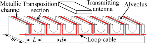
Fig. 1 Block diagram of loop-cable, long stator and transmitting antenna

In this work, a new kind of method is introduced to extract the train’s running direction based on the differential of the sampling signal and the XOR (exclusive OR) pulses. The classical differentiator just uses the inertia process to get the approximate differential coefficient, which has the shortage of amplifying the signal noise, and it cannot be used in the practical system.

The filtering method based on the tracking- differentiator has the advantages of real-time and high efficiency. Also, it can effectively extract the differential input signal. A new kind of discrete tracking differentiator is constructed in this work, which provides a good performance of filtering, and needs only relatively small calculation.

2 Positioning system based on loop-cable

The positioning system affords the position and direction information for the traction system and the operation control system of the mid-speed maglev train. Here, the trackside signal receiving and processing part is the core of this technology. It is composed of the loop-cable laying on the track, the impedance matching and pretreatment unit, and the signal processing case, as shown in Fig. 2. The loop-cable is used to induce the alternating signal sent by the on-board antenna, which is modulated by the relative position of the train. The impedance matching and pretreatment unit has two functions: filtering the received signal by the loop-cable, and preventing signal distortion caused by electromagnetic wave reflection. The signal processing case includes the analog unit and the digital unit. The former is responsible for signal amplification, filtering, and envelop detection; the latter is responsible for digital filtering, converting the amplitude into the position information by looking up, and data communication protocols.

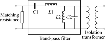
Fig. 2 Impedance matching and band-pass filter

2.1 Impedance matching and pretreatment

As the frequency of the electromagnetic wave is relatively low, the influence of the transmission on the signal amplitude and phase is small and the design of the circuit does not need to consider the length of the line. As the frequency increases, the distribution characteristic of the loop-line will gradually manifest, and the magnitude and the phase of the transmitting signal will be affected. To prevent or decrease the signal distortion, the load should match with the characteristic impedance of the loop-cable. Therefore, matching resistances are required at the original and terminal ends, as shown in Fig. 2.

As for the secondary motor, the long stators are installed along the centre line of the track, and the loop- cable is embedded in the long stators. This structure minimizes the effect of the suspension magnetic field on the loop-cable, but the magnetic field of the traction during traveling would produce relatively strong electromagnetic interference. This interference may be easily transferred into the post-processing circuit, which would degrade the position estimation, and even get IC (integrated circuit) damaged. So, effective measures should be taken to enhance the ability of anti- electromagnetic interference of the system [5–6].

For the above reasons, a passive band-pass filter is designed, as shown in Fig. 2, which can effectively limit the excessive signal saturation and the impact on the circuit caused by low-frequency harmonics. The capacitor C1 and the adjustable inductor L1 with a ferrite core make up a series of resonant circuit, and the resonant frequency is the operating frequency. The capacitor C2 and the inductor L2 make up a parallel resonant circuit, and its terminal acts as the output of the filter. Thus, the resonant split-voltage band-pass filter is designed.

2.2 Analog signal processing unit

As the transmitting antenna moves along the loop- cable, the relative position between the antenna and the long stator is converted into the change of the amplitude of the received signal by the loop-cable. Therefore, to obtain the accurate position, it is necessary to detect the amplitude without interference. It should be noted that, although the transmitting antenna is fixed on the bogie under the vehicle, the height between the transmitting antenna and the loop-cable may still change within a dynamic range as the suspension height changes. When the height increases, the amplitude of the received signal becomes smaller; when the height decreases, the amplitude becomes larger. To minimize this effect, the double loop-cable structure shown in Fig. 3 is employed, where Loop A and Loop B stagger half of one cross cycle. By the amplitude division operation of the two received signals, the effect caused by the suspension height variation can be weakened [7–9].

In the analog signal processing unit, the amplitude of the received signal with fixed frequency is demodulated by a circuit shown in Fig. 4.

In addition, to detect the amplitude of the received signal, the analog unit can also generate a pulse signal using XOR process, which is needed in direction identification, as shown in Fig. 5.

2.3 Digital signal processing unit

Digital signal processing unit is used to calculate the relative position and to obtain the running direction using the input signals (the sample value of the amplitude and the XOR pulse). Its specific features include the following items.

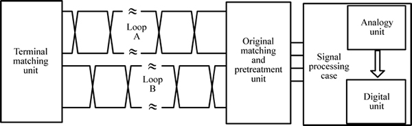
Fig. 3 Block diagram of trackside part

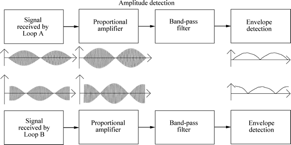
Fig. 4 Amplitude demodulation circuit

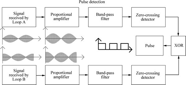
Fig. 5 XOR pulse generating circuit

(1) Pulse counting

This unit receives the pulse signal sent by the analog unit, and it counts the number. One pulse period represents the length of two alveoli.

(2) Position estimation within one alveolus

Pulse counting could only reach the accuracy of two alveoli. In order to meet the requirement of high accuracy of relative position (2 cm), the positioning system should be able to identify the position within one alveolus; therefore, the digital unit must have the functions of sampling the amplitude, digital filtering, and converting the filtering result into position information by looking up.

(3) Direction identification

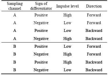
The direction identification is not only a basic function of the pulse counting circuit, but also the necessary for the traction control. The direction should be identified within two alveolus. Due to the symmetrical laying of the loop-cable, the direction cannot be obtained directly. However, considering the corresponding relationship of the pulse signal and the amplitude signal, which is shown in Fig. 6, the direction can be inferred accordingly. For example, when the train runs forward, the differential value of the signal in Channel A is calculated. It can be found that when the differential value is bigger than zero, it corresponds to the high level of the pulse signal. On the contrary, as the differential value is less than zero, it corresponds to the low level of the pulse signal. The detailed method is given in Table 1.

3 Tracking-differentiator

The method based on the tracking-differentiator filtering has the advantages of real-time and high efficiency. Also, it can effectively extract the differential input signal for direction identification.

3.1 Classical differentiator equations

In classical control theory, to obtain the differential value of a given signal, the following method is often used [10–12]:

  (1)

In fact, Eq. (1) uses the first-order inertial process 1/(Ts+1) instead of the delay process exp(–Ts). If the inertial delay signal is close enough to the output signal, the differential value could reach high accuracy. However, if a Gaussian white noise ω(t) is superimposed

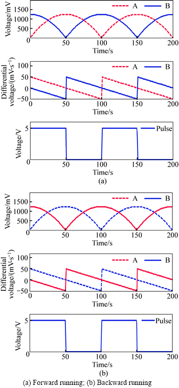
Fig. 6 Amplitude signals, their differential values and pulse signal:

Table 1 Method of direction identification

upon the input signal x(t), the approximate differential expression is as follows:

                (2)

where  is the output of the first-order inertial process, and it could be expressed as [11]

           (3)

In fact, the first item of the above equation could meet As ω(t) is the white noise over a wide frequency range and its mean value is zero, the second item of Eq. (3) is almost zero. Thus, Eq. (2) becomes

     (4)

We could find in the above equation that the output signal y(t) is composed of the differential x′(t) and the amplified noise of 1/T times. When the value of T is very small, the noise would be amplified very seriously and the differential signal may be submerged completely, resulting in the noise amplification effect of the classical differentiator.

Based on the idea of extracting the “differential”, HAN [11] proposed a dynamic structure of a second- order tracking-differentiator, which is based on the optimal second-order integrated function. This is a form of a switch structure, which is also called “bang-bang” control in optimal control theory. But its discrete form is likely to cause divergence [12]. To solve this problem, the linear control region around the switching curve is drawn. The simulation results show that the tracking performance and the differential quality are sensitive to the size of the region. Whether or not the linear region can be determined in theoretical method has an important guiding significance for the discrete tracking- differentiator [11,13].

The track-differentiator that HAN proposed uses the method of the same time zones to determine the control strategy [12]. The general form of the optimal control function is given, which is actually a kind of nonlinear boundary transformation. It includes three situations: (1) the switching curve, (2) the boundary where the state variables could reach within one step, and (3) the boundary where the control variable takes zero. This kind of non-linear transformation contains some square root operations, which causes a certain complexity to the control algorithm. To solve this problem, in this work,state backtracking method is used to seek the boundary characteristic points where the control variable does not exceed the limit value. Thus, the linear region and the reachable region are distinct. According to the features of the linear region, the control variable is determined using the method of linear proportion, and the piecewise linear function is constructed by using the characteristic points. This algorithm only uses the method of constant value comparison on the boundary to determine whether the state point is located within the linear region or not. Thus, the computation of nonlinear transformation is removed and the square root operation is avoided. XIE et al [13–14] introduced this new kind of tracking- differentiator and applied it to the loop-cable positioning system.

3.2 Discrete second-order nonlinear track- differentiator based on boundary characteristic curves

3.2.1 Boundary curves and control characteristic curve

First of all, the second-order continuous-time system is studied:

                     (5)

where  is the differential of x₁,  is the differential of x₂, and u is the control variable.

The initial state is  and the permissible control domain is |u|≤r. r is the boundary of u and r>0. The problem is how to find the time optimal control to minimize the system performance. For the system (5), there exists one optimal control strategy, which could make arbitrary point M (x₁₀, x₂₀) in the state space reach the origin using at most one switching. All the control switching points compose the switching curve in Eq. (6), which is shown in Fig. 7. The switching curve is [11, 15–16]:

                  (6)

In reference from the optimal control theory, the solution of the above control problem is as follows:

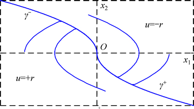
Fig. 7 Switching curve

     (7)

When the point locates above the switching curve, the control variable takes the negative limit value u=–r; when it locates below the curve, the control variable takes the positive limit value u=+r. When the state point reaches the switching curve, the control variable changes symbols, taking +r and –r, respectively. However, in the discrete system, the control variable is between ±r and it must take the value of zero for at least once. The points that the control variable takes zero form the control characteristic curve. The region that the control variable takes between ±r is denoted as Ω. Obviously, the region must be near the switching curve. Therefore, we only need to find the boundaries of the region Ω and control characteristic curve.

The discrete form of the double integration system is as follows:

                (8)

where h is the sample interval, and x₁(k) and x₂(k) are the state variables at the time T=kh. Equation (8) could also be expressed as

                     (9)

where

After k+1 steps, the state reaches the origin, and the control sequence is represented as u(0), u(1), …, u(k–1), u(k). Starting from the initial state the state turns to be

          (10)

As the final state reaches the origin, i.e. X(k+1)=0, the initial point should satisfy the following equation:

               (11)

Using Eq. (11), the two boundaries of the region Ω and the control characteristic curve can be found. They satisfy the following conditions:

(1) One of the boundaries of Ω is the switching curve Г_A. There is a sequence of points. The control variable of these points takes the limit value, i.e. u=+r or u=–r, and the state variable could finally reach the origin. Assume that the point sets are {a_+k} and {a_–k}.

(2) The other boundary is denoted as Г_B. If the initial point lies on it, the control variable should firstly take u=–r, and then u=+r, or the control variable firstly takes u=+r, and then u=–r, and thus the state variable could reach the curve Г_A. Assume the point sets are {b_+k} and {b_–k}.

(3) The control characteristic curve is denoted as Г_C. If the initial point lies on it, the control variable should firstly take zero, and then u=+r or u=–r, and thus the state variable could reach the curve Г_A. Assume that the point sets are {c_+k} and {c_–k}.

The state space can be divided into two regions: one is Ω and the other is the remaining part (R²–Ω), which is denoted as  Any point on the state space could reach the origin with one control strategy. The region Ω can be divided into two parts: one is the region in which the initial point could reach the origin within two steps, denoted as Ω₂; the other is outside the region Ω₂ in which the initial point could reach the origin within at least three steps. According to the characteristics of the region Ω and the optimal control theory, when the state point locates outside Ω, the control variable takes u=±r. Thus, within limited steps, the state variables could be closer to the boundary curve Г_B. As the state variables are inside the region Ω, the appropriate choice of the control variable should be |u|A [11, 15].

Then, the boundaries (Г_A, Г_B and Г_C) can be calculated (Fig. 8) and its mathematical expression can be given:

(1) The boundary curve Г_A will be figured out. The {a_+k} is the set that the points in it could reach the origin by taking u=+r. Assuming that the state variable reaches the origin after k+1 steps, i.e. X(k+1)=0, there is u(i)=r, i=0, 1, …, k. By Eq. (11), the following equation can be obtained:

                        (12)

Thus,

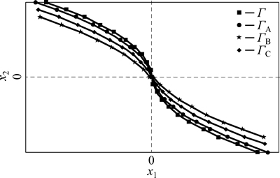
Fig. 8 Switching curves of continuous and discrete system, Г_B and Г_C

          (13)

Eliminating the variable k in Eq. (13), it gives

                             (14)

Equation (14) is the curve where the set {a_+k} locates.

Similarly, the curve equation where the set {a_–k} locates is given as

                            (15)

Equations (14) and (15) can be combined into one equation:

              (16)

Secondly, the boundary curve Г_B can be determined. For the set {b_+k}, assuming X(k+1)=0, there is u(0)=–r, u(i)=+r, i=1, 2, …, k. By Eq. (11), the following equation can be obtained:

    (17)

Eliminating the variable k in Eq. (17) gives

 (18)

This equation is the curve where the set {b_+k} locates.

(2) The curve equation where the set {b_–k} locates is as follows:

                       (19)

Equations (18) and (19) can be combined into one equation:

            (20)

where is the sign function.

(3) The boundary curve Г_C can then be figured out. For the set {c_+k}, assuming X(k+1)=0, there is u(0)=0, u(i)=+r, i=1, 2, …, k. From Eq. (11), one obtains

         (21)

Eliminating k in Eq. (21) gives

                             (22)

Similarly, the curve equation where the set {c_–k} locates is as follows:

                            (23)

Equations (22) and (23) can be combined into one equation:

             (24)

So, all the boundaries of the region Ω and the control characteristic curve are obtained, namely:

         (25)

3.2.2 Control strategy

The region Ω where the control variable takes between –r and +r has been identified in Section 3.2, and the region Ω–Ω₂ where the state variables could not reach the origin within two steps has also been considered. Then, in the state space R², if the state variables are included by Ω, the control variable takes the limit value (+r or –r). So, we consider the value of the control variable in the region Ω. Suppose that the point M(x₁,x₂) locates in the fourth quadrant (x₁>0, x₂<0), and then make an auxiliary line crossing M (x₁, x₂), as shown in Fig. 9. It intersects the boundary curves and the characteristic curve at the points A, B and C, which correspond to the x₁ axis coordinates: x_A, x_B, x_C. The control variable takes u=+r, –r, 0 separately, if (A, B, C) are the initial points. If the point M(x₁, x₂) does not locate between the points A and B, the control variable takes the limit value. Otherwise, because of the presence of the control characteristic curve Г_C, it is reasonable to consider that M (x₁, x₂) locates in the interval A and C, or C and B. So, we take the control variable u as linear value, namely:

If  then and u=α·r

Otherwise, if then  and u=–α·r

Supposing that the point M(x₁, x₂) locates in the second quadrant, the similar control strategy could be obtained.

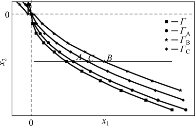
Fig. 9 Auxiliary line crossing M(x₁, x₂) intersecting boundary curves and characteristic curve

Obviously, if the point M(x₁, x₂) locates in the first and third quadrant, it is not in Ω, and u=–r·sgn(x₁+hx₂) in the condition that M(x₁, x₂) could not reach the origin within two steps. If the point M(x₁, x₂) could reach the origin within two steps, the initial state variable X(0) and the associated control variable must satisfy the equation set as follows:

                        (26)

Supposing x₁(2)=x₂(2)=0, the above equation set can be expressed as

        (27)

And it could be calculated as

                     (28)

In fact, because x₁(1)+hx₂(1)=0, it can be inferred that

                      (29)

So, the control strategy of reaching the origin within two steps can be expressed as

The initial points that could reach the origin forms the region Ω₂, which is surrounded by the parallel lines x₁+hx₂=±h²r and x₁+2hx₂=±h²r. It is a kind of diamond region connected by four points: (–h²r, 0), (–3h²r, 2hr), (h²r, 0), (3h²r, –2hr). So, we could get the detailed description of the track differentiator algorithm:

Step 1: Set y₁=x₁+hx₂, y₂=x₁+2hx₂. If |y₁|>h²r or |y₂|>h²r, i.e. it could not reach the origin within two steps, go to the Step 1; or go to Step 5.

Step 2: If x₁·x₂≥0, then u=–r·sgn(x₁+x₂), and go to  Step 3.

Step 3: Calculate the boundary of Ω, and then go to  Step 4:

Obviously, x_ACB.

Step 4: If |x₁|≥x_B, then u=–r·sgn(x₁).

If |x₁|≤x_A, then u=r·sgn(x₁). Otherwise, calculate the coefficient: and

If |x₁|≤x_C, then u=–r·α·sgn(x₂); or u=+r·β·sgn(x₂). There is  and  i.e.

Step 5: If it could reach the origin within two steps,

The above function could be denoted as u=fast(x₁, x₂, r, h). In fact, for a given input signal sequence {v(k), k=1, 2, …}, we could obtain the general form of the tracking differentiator [11]:

          (30)

where the parameter r is the gain of the control variable (or called as fast factor), c₀ is the filter factor and h is the sampling interval.

4 Application to signal processing of loop- cable

4.1 Signal filtering of loop-cable

The variation of the suspension height would cause the amplitude of the received signal to fluctuate. In addition, the mid-speed maglev train adopts the technology of passive levitation and guidance, which would make the transmitting antenna sway from side to side with the bogies. In Section 2, the amplitude division operation was proposed to solve this problem. However, to make the position estimation more precise, we need to select one appropriate digital filter to treat the signal in advance. Figure 10 shows the signal waveform received.

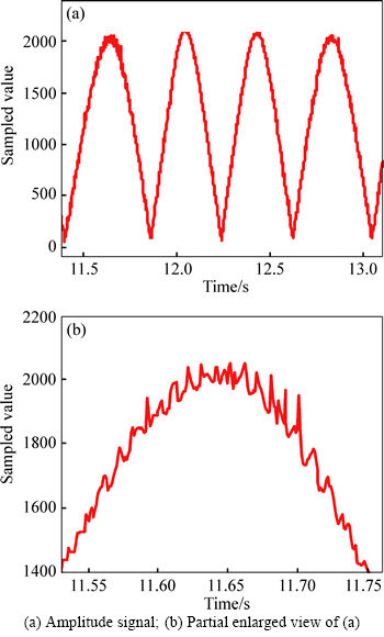
Fig. 10 Untreated received sample signal:

The algorithm described in Section 3 can be used. The sample interval is h=0.001 s. Take the filter coefficient c₀=5. Generally, when the amplitude of the input signal is A and the frequency is ω, it is recommended to take the fast factor as r=A·ω/(c₀·h). Here, the fast factor in the system is r=880000. The filtered result is shown in Fig. 11.

From Fig. 11, it can be seen that the track-differentiator could track the input signal and has the ability to do the filter work. The interference caused by the variation of the transmitting antenna could be effectively suppressed. But the filtering ability of the track-differentiator is related with phase delay, i.e. the stronger the filtering ability is, the greater the phase delay will be. So, it is recommended to select an appropriate filter factor, which could not only meet the filtering requirement, but also cause little phase delay.

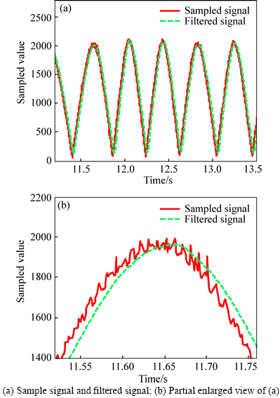
Fig. 11 Sample signal and filtered signal:

4.2 Extraction of signal differential

The digital signal processing unit identifies the direction using the sample signal differential and the XOR pulse. The track-differentiator not only has a strong filtering ability, but also can extract the differential of the input signal, as shown in Fig. 12.

Actually, the direction identification does not care about the value, but it needs to obtain the symbol of the signal, i.e., positive or negative. Therefore, the differential can be done by the process of digital zero-crossing comparator. If the value is greater than zero, the output is in high level; otherwise, the output value in is low level (zero). The result is shown in Fig. 13.

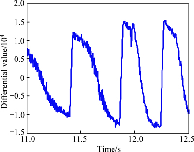
Fig. 12 Extraction of input differential

As can be seen from Fig. 13, there are fluctuations near the zero crossing, which indicates that the output is too sensitive and susceptible to interferences. In order to enhance the inertia of the digital zero-crossing comparator, a hysteresis function is embedded. A satisfactory result is obtained in Fig. 14.

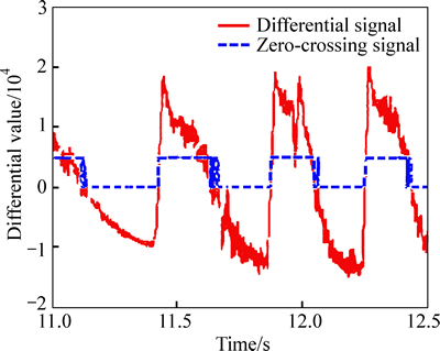
Fig. 13 Differential and output after zero-crossing comparator

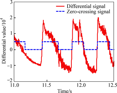
Fig. 14 Differential and output after zero-crossing comparator with hysteresis

5 Conclusions

The positioning system is described based on the induction loop-cable of the mid-speed maglev train, and the trackside part and the processing part of its received signal are focused on, which includes the impedance matching and pretreatment unit, the analogy signal processing unit and the digital signal processing unit. The basic functions of each unit are introduced. As the received signal could be easily affected by the height change of the transmitting antenna, which may decrease the system accuracy, the discrete second-order nonlinear track-differentiator based on boundary characteristic curves is used for filtering. Meanwhile, in order to detect the running direction of the train, the method based on the sampling signal differential coefficient and XOR pulse is proposed. The experimental result shows that the differentiator is able to extract the signal differential and the direction could be detected accurately within one unit ring.

References

[1] WU X M. Maglev train [M]. Shanghai, China: Shanghai Science and Technology Publishing House, 2008: 1808–1811. (in Chinese)

[2] LEE Hyung-woo, KIM Ki-chan, LEE Ju. Review of maglev train technologies [J]. IEEE Transactions on Magnetics, 2006, 42(7): 1917–1925.

[3] LI Yun, LI Jie, ZHANG Geng. Disturbance decoupled fault diagnosis for sensor fault of maglev suspension system [J]. Journal of Central South University, 2013, 20(6): 1545–1551.

[4] ZHOU Hai-bo, DUAN Ji-an. Levitation mechanism modeling for maglev transportation system [J]. Journal of Central South University of Technology. 2010, 17(6): 1230–1237.

[5] BELLAN P M. Simple system for locating ground loops [J]. Review of Scientific Instruments, 2007, 78: 065104.

[6] SKIBINSKI G. Design methodology of cable terminator to reduce reflected voltage on AC motors [C]// Conf Rec IEEE-IAS Annu Meeting. San Diego, CA, USA, 1996: 153–161.

[7] THEODOULIDIS T, BOWLER J. Eddy-current interaction of a long coil with a slot in a conductive plate [J]. IEEE Transaction on Magnetics, 2005, 41(4): 1238–1247.

[8] MISRON N, YING L Q, FIRDAUS R N, ABDULLAH N. Effect of inductive coil shape on sensing performance of linear displacement sensor using thin inductive coil and pattern guide [J]. Sensors, 2011, 11: 10522–10533.

[9] NORHISAM M, NORRIMAH A, WAGIRAN R, SIDEK R M, MARIUN N, WAKIWAKA H. Consideration of theoretical equation for output voltage of linear displacement sensor using meander coil and pattern guide [J]. Sensor and Actuators A, 2008, 147: 470–473.

[10] DAI C H, LONG Z Q, XIE Y D. Research on the filtering algorithm in speed and position detection of maglev trains [J]. Sensors, 2011, 7: 7402–7218.

[11] HAN J Q. Auto disturbances rejection control technique [J]. Front Sci, 2007, 1: 24–31.

[12] GUO B Z, ZHAO Z L. On convergence of tracking differentiator [J]. International Journal of Control, 2011, 84(4): 693–701.

[13] XIE Y D, LONG Z Q. A high-speed discrete tracking-differentiator with high precision [J]. Control Theory Appl, 2009, 26: 127–132.

[14] XIE Yun-de, LONG Zhi-qiang, LI Jie. Analysis of the second-order nonlinear discrete-time tracking-differentiator as a filtering [J]. Information and Automation, 2008: 785-789.

[15] XIE Y D, LONG Z Q, LI J, LUO K. Research on a new nonlinear discrete-timetracking-differentiator filtering characteristic [C]// Proceedings of the 7th World Congress on Intelligent Control and Automation, WCICA 2008. Chongqing, China, 2008: 6750–6755.

[16] XUE Song, LONG Zhi-qiang, HE Ning, CHANG Wen-sen. A high precision position sensor design and its signal processing algorithm for a maglev train [J]. Sensors, 2012, 12: 5225–5245.

(Edited by YANG Bing)

Foundation item: Project(11226144) supported by the National Natural Science Foundation of China

Received date: 2014-12-02; Accepted date: 2015-03-19

Corresponding author: DOU Feng-shan, PhD Candidate; Tel: +86-731-84516000; E-mail: dfs5460@126.com