J. Cent. South Univ. (2012) 19: 2142-2151

DOI: 10.1007/s11771-012-1257-1

Vision-based behavior prediction of ball carrier in basketball matches

XIA Li-min(夏利民), WANG Qian(王千), WU Lian-shi(吴联世)

School of Information Science and Engineering, Central South University, Changsha 410075, China

? Central South University Press and Springer-Verlag Berlin Heidelberg 2012

Abstract: A new vision-based approach was presented for predicting the behavior of the ball carrier—shooting, passing and dribbling in basketball matches. It was proposed to recognize the ball carrier’s head pose by classifying its yaw angle to determine his vision range and the court situation of the sportsman within his vision range can be further learned. In basketball match videos characterized by cluttered background, fast motion of the sportsmen and low resolution of their head images, and the covariance descriptor, were adopted to fuse multiple visual features of the head region, which can be seen as a point on the Riemannian manifold and then mapped to the tangent space. Then, the classification of head yaw angle was directly completed in this space through the trained multiclass LogitBoost. In order to describe the court situation of all sportsmen within the ball carrier’s vision range, artificial potential field (APF)-based information was introduced. Finally, the behavior of the ball carrier—shooting, passing and dribbling, was predicted using radial basis function (RBF) neural network as the classifier. Experimental results show that the average prediction accuracy of the proposed method can reach 80% on the video recorded in basketball matches, which validates its effectiveness.

Key words: covariance descriptor; tangent space; LogitBoost; artificial potential field; radial basis function neural network

1 Introduction

It is revealed that the introduction of the digital video technology into the field of sports training can contribute to the efficiency of training by the long-term practice and researches of the sports experts. Therefore, how to make use of the techniques, such as computer image processing, and video analysis to ameliorate the sports training, has become the current hot spot [1-4]. The main purpose of the sports video analysis is to realize the scientific training through analyzing the videos shot in the training and match and utilize the correlation of video images in time and space to obtain a variety of kinesiology parameters and the information, which sportsmen and coaches are interested in. As a prevailing and typical team sport, the result of basketball match depends on the close cooperation of the players, which further hinges on the decision of the ball carrier. Therefore, it is instructive to make analysis and prediction for the ball carrier’s behaviors—shooting, passing and dribbling.

The behavior prediction for the ball carrier in basketball matches is a complex behavior analysis at the high level of human behavior analysis. It requires the recognition of the ball carrier’s behaviors as well as the consideration of all kinds of relations between the ball carrier and other players, the basket of the opposing team, etc. Currently, a Chinese research focused on human behavior recognition but the researches on behavior prediction are relatively insufficient. DUQUE et al [5] proposed an abnormal behavior prediction method based on N-ARY trees classifier and adaptative dynamic oriented graph (DOG) [6] with greater real-time property. In reality, the prediction of human behavior usually has more significance than behavior recognition. For instance, if the smart surveillance systems installed in the security-sensitive places, such as banks, airports and government buildings, can sound the alarm to the security guards when detecting suspicious security problems, i.e. predicting the criminal behaviors, both the occurrence of crimes and the huge input of human, material and financial resources can greatly decrease. In basketball matches, the progress of the matches can be predicted, if the behaviors of ball carrier can be learned in advance.

A novel prediction method for the behavior of ball carriers in basketball matches was proposed. Aiming at the cluttered background, the fast motion of the sportsmen and the low resolution of the head images in the basketball match videos, the covariance descriptor was adopted to fuse multiple visual features of the head region, which can be seen as a point on the Riemannian manifold. Then, for the purpose of determining the vision range of the ball carrier, the covariance descriptor was mapped to the tangent space and the head pose recognition was completed through the trained multiclass LogitBoost directly in this space. The artificial potential field (APF)-based information was introduced to describe the court situation of all players within the ball carrier’s vision range, and the prediction for ball carrier’s behavior was completed through the classifier based on RBF (radial basis function) neural network.

2 Vision range determination of ball carrier

Before the vision range of the ball carrier is determined, it is assumed that the players of both sides have been detected and the marking of their positions on the court has been finished. In order to determine the ball carrier’s vision range, it is needed to further decide the head pose of the ball carrier, i.e. classifying the yaw angle of his head into one of the eight orientations, as illustrated in Fig. 1. Most existing head pose recognition algorithms aim at human-computer interaction with high-resolution images [7-9], thus the head and face features can be effectively extracted. In contrast, limited features can be extracted in the videos of basketball match due to low resolution, noise, motion blur and low proportion of the player’s head to the whole image.

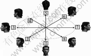
Fig. 1 Eight head poses

TUZEL et al [10] proposed a robust human detection method resistant to the environmental changes. They considered human detection as classifying the foreground (human) from the background and demonstrated the promising experimental results based on the INRIA (Institut National de Recherché en Informatique et en Automatique) and DaimlerChrystel databases. In order to detect the head of ball carrier and distinguish eight head poses simultaneously, the two- class classification in Ref. [10] was extended into multi- classification.

2.1 Head feature extraction based on Riemannian manifolds

For each training sample, N square areas of the same size are first extracted, which may partially overlap with others. Then, a 12-dimensional feature vector f=  [x y R G B I_x I_y O G{0, π/3, π/6, 4π/3}] is computed for each pixel within each extracted square area, where x and y are the pixel coordinates; R, G and B are three color channels; I_x and I_y are first order derivatives; O is gradient orientation; G{0, π/3, π/6, 4π/3} respectively denote the values responding to the Gabor filter with dimension 2×4, sinusoidal frequency 16 and orientations {0, π/3, π/6, 4π/3}. The reason for extracting the color channels is to capture the different proportions of the skin area to non-skin area within the head of ball carrier in different yaw angles (e.g. front and back) and the purpose of computing response to the Gabor filter is to extract the head texture feature. The covariance descriptor for each region is defined as

                                   (1)

where  is the mean of the feature vectors computed for all the pixels within the r-th area of the k-th training sample;  is the amount of pixels in the r-th area of the k-th sample;  is the feature vector of the i-th pixel in the r-th area of the k-th training sample. The covariance descriptor  is a symmetric matrix, the diagonal entries of which represent the variance of each feature, and the nondiagonal entries are their correlations. TUZEL et al [11] proposed a fast calculation of covariance descriptor for a given rectangular area through integral image. With this method, the covariance descriptor of any rectangular region can be computed in o(d²) time, where d denotes the dimension of the feature vector for each pixel. In the experiment, this method is adopted to accelerate the computation of covariance descriptor for each area.

Since covariance descriptor doesn’t form a vector space, it is inappropriate to use classical machine learning methods to learn a classifier. Mathematically, the covariance descriptor is a symmetric and semi- positive definite matrix. FLETCHER and JOSHI [12] pointed out that a set of n×n symmetric semi-positive definite matrices constitute a convex cone in the n(n+1)/2-dimensional linear space. The variances of the computed image features are unlikely to be zero, so it is only necessary to take nonsingular covariance matrix (i.e. symmetric and positive definite) into consideration. Most of all, the set of symmetric positive definite matrices correspond to the interior of a convex cone, which is a differentiable manifold. Therefore, it is feasible to adopt differential geometry as the following solution. PENNEC et al [13] proposed an affine-invariant measurement in differentiable manifold. The main idea is that from any point X on the Riemannian manifold M, it is possible to construct a tangent space S_x, which is diffeomorphic with the manifold M. The tangent space is a linear one consisting of all the tangent vectors of a point on the manifold. As for the vector V in the tangent space S_x, it can be mapped into the equi-long and equi-directional geodesic starting from the point X on the manifold through exponential mapping  associated to the Riemannian metric, where X is a symmetric matrix.

                           (2)

While the geodesic from X to point Y on the Riemannian manifold can be mapped to V in the tangent space by the inverse of exponential mapping-logarithm mapping:

                            (3)

The exponential mapping and logarithm mapping mentioned above constitute the homeomorphic mapping between tangent space S_x and Riemannian manifold M. The points on Riemannian manifold can be projected to the tangent space S_x through this homeomorphic mapping. Therefore, by applying this affine-invariant measurement to the differentiable manifold constituted by covariance descriptors to form Riemannian manifold, all the points on this manifold are mapped to the tangent space and the head pose is recognized in this linear space through the classifiers based on machine learning.

Because it is possible to construct a tangent space from any point X on the manifold M, there exist innumerable tangent spaces. So, it is necessary to define a uniform tangent space as the mapping space for the points on the Riemannian manifold. Generally, the mean of a cluster of points (Y₁, Y₂, …, Y_n-1, Y_n) in the Euclidean space can be regarded as the best representative for them. Similarly, for a cluster of points (X₁, X₂, …, X_n-1, X_n) on Riemannian manifold, the tangent space constructed by the mean of them can be the optimal approximation of the manifold. The Karcher mean of points on the Riemannian manifold is the point on M that minimizes the sum of squared Riemannian distances, as proposed in Ref. [12]:

                                                 (4)

where the computed mean has the minimal sum of squared distance with the point set {X_i}_{i=1, …, n} and the squared distance between two points on Riemannian manifold is

                                   (5)

For the convex cone manifold formed by the covariance descriptors, the Karcher mean μ is unique, which can be obtained through the gradient descent

procedureand μ^t is the

Karcher mean point obtained after the t-th iteration. The iteration stops when  is satisfied. Finally, the orthonormal coordinates of a tangent vector V in the tangent space S_μ at the Karcher mean μ is given by the vector operator:

                                                     (6)

where I is the identity matrix, and the vector operator at I is defined as

       (7)

2.2 Vision determination based on multiclass LogitBoost

For all kinds of collected training samples, the orthogonalized feature vectors in the tangent space S_μ at the Karcher mean μ are extracted for each area of each sample according to the method introduced in Section 2.1 and they are denoted as the set  1≤r≤N, where γ and k are the amounts of regions and samples, respectively. Then, a multiclass LogitBoost is built for each area taking A_r as the training set. As for the test sample, the classification result is determined by voting of all multiclass LogitBoosts.

2.2.1 Training of classifier

The procedure of training the classifier is as follows:

Input the set of head training samples of different yaw angles in different conditions and non-head training samples  Y₁)… Y_i)… Y_n) where  denotes covariance descriptor corresponding to the k-th region in the i-th training sample; Y_i{1, 2, 3, 4, 5, 6, 7, 8, 9} denotes the class labels of the different head poses in Fig. 1 and the non-head class label.

Step 1: Compute the Karcher mean μ^k of the covariance descriptors corresponding to the k-th region of all head training samples through gradient descent

procedure       and map all the

training data to the tangent space at the Karcher mean by the logarithm mapping  and orthogonalize them, i.e.

Step 2: Initialize weights 1/N, i=1, …, n,  .

Step 3: Get the weak classifiers through iteration

for l=1, 2, …, L do

for j=1, 2, …, 9 do

1) Compute the response values and weights:

where

2) Fit the weak classifiers by weighted least-square regression;

3) Update  

where  and g_ld is the weak learner.

4) Update

5) Save

End

End

Step 4: Save {F₁, …, F₉}

L is the total number of iteration in the LogitBoost training phase, L=max_i{a(j)≥τ_accuracy(a_l(j)-a_l-1(j))≤ a_background≥τ_background, j{1, …, 8}}. Specifically, a_l(j) is the accuracy of the j-th strong classifier after the l-th iteration, a_l(j)-a_l-1(j) represents the improvement of the j-th strong classifier accuracy between two consecutive iterations, and a_background is the accuracy of the strong classifier of background.

2.2.2 Vision range determination

During the shift of the scanning window, the covariance descriptor for each region within this window is computed and mapped to the tangent space at mean point μ^k by Eq. (3) and then orthogonalized, respectively. The feature vectors extracted from the scanning process are input to the trained multiclass LogitBoosts and the head pose class is determined by counting the results of all the small regions according to

(k=1, …, 9)                                                                     (8)

where  is the sum of the regions voting for class k, and L_i is the class label of the i-th region determined by the corresponding LogitBoost.

After the recognition of the ball carrier’s head pose, his vision range can be further determined. In Fig. 2, the ball carrier’s vision range is highlighted.

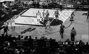
Fig. 2 Visual field of ball carrier

3 Behavior prediction of ball carrier

After player detection and head pose recognition for the ball carrier, the player distribution of both sides on the court and the vision range of the ball carrier can be obtained. In this section, a prediction algorithm is proposed for the ball carrier’s behavior based on artificial potential field (APF) and RBF neural network.

In a basketball match, the ball carrier can choose shooting, passing or dribbling the ball. The ball carrier’s choice is jointly determined by multiple factors, such as the role who plays in the team (forward, center or rearguard), the distance away from the basket of the opposing team, the court position of the other four teammates and the players of the opposing team as well. This is an inherently complicated decision-making process. Therefore, it is reasonable to treat behavior prediction of the ball carrier as a three-classification problem considering multiple factors. In this section, the APF-based information is applied to model the condition of each player just before the moment the ball carrier carries out his determination. Then, a feature vector is constructed to describe the scene. Finally, this feature vector is further input into the trained RBF neural network and the behavior prediction is completed by the network.

3.1 Information quantity based on APF

In basketball matches, the players can be divided into one dribbler and the others without ball. The information quantity of the players can be described by APF [14-15]. The APF of the player p is

U_APF(p)=U_goal(p)+U_obs(p)                                                         (9)

where U_APF(p), U_goal(p) and U_obs(p) are artificial potential field, the attractive potential generated by the target and the repulsive potential generated by the barriers, respectively. The target here is the basket of the opposing team and barriers are the players of the opposing team; p is the position of the player. The attractive potential is described as

                    (10)

where (p-x_goal) is the distance between the ball carrier and the basket of the opposing team. The smaller the value is, the bigger the attractive potential is, which implies that the player is closer to the basket of the opposing team; on the contrary, smaller attractive potential indicates farther distance between the player and the basket of the opposing team.

The repulsive potential is

          (11)

where ρ is the distance between the player p and his nearby player of the opposing team and ρ₀ is a distance threshold, over which the player of the opposing team doesn’t impose any influence on the player x. It is necessary to consider multiple repulsive potentials  U_obs(     p) when computing the artificial potential field for a player, if there exist more than one players of the opposing team within the valid sphere (ρ≤ρ₀).

Here, it needs to be emphasized that k_p in Eq. (10) is a positive gain indicating the player’s scoring ability. As for the players of the offensive team, different roles have different scoring abilities. So, k_p values are different for different roles. Similarly, k_d in Eq. (11) is a negative gain reflecting the tackling ability. As for the players of the defensive team, different roles have different tackling abilities. Therefore, k_d values are also different for different roles.

Since it is impossible to appraise the role of the player from the image, an algorithm updating k_p and k_d according to the statistics of tackling and shooting is proposed. At the beginning of the training phase,  and  are initialized with the constant values α and β, respectively, which assumes that each player has equal ability. Here A and B are the team labels. As the match progresses, k_p is updated according to Eq. (12) when the ball carrier shoots the basketball successfully:

k_{p, carrier}=k_{p, carrier}+τ, η_a≤k_p,carrier≤θ_a                                        (12)

If the ball carrier fails,

k_{p, carrier}=k_{p, carrier}-τ, η_a≤k_p,carrier≤θ_a                                        (13)

In the match,  needs to be updated on the occasion that the player B_i has successfully tackled the ball carrier of team A:

                                       (14)

If the player B_i fails,

                                        (15)

In a similar way, when the player A_i of team A tackles the ball carrier of team B successfully:

                                         (16)

If the player A_i fails,

                 (17)

where θ_d and η_d are the upper and lower limits of the tackling ability, while θ_a and η_a are the upper and lower limits of shooting ability, respectively. Variables γ and τ are the step length of the scoring ability and tackling ability, respectively.

3.2 Behavior prediction based on RBF network

The behavior prediction of the ball carrier can be considered as a highly nonlinear complex process affected by multiple factors with lots of uncertainties. To solve these problems, neural network is introduced in this work. Neural network has the properties of self- organization, self-learning, self-adaptation and nonlinearity, which is capable of tackling the intrinsic elusive regularity of the complex system and suitable for the modeling of nonlinear system. As a widely-used feed-forward neural network, RBF network can achieve optimal approximation and global optimum, which has a better performance than the traditional BP network in accuracy and convergence velocity for nonlinear system. Therefore, the RBF network is the right choice for the behavior prediction model.

The RBF neural network is typically a three-layer feed-forward network consisting of an input layer, a hidden layer and an output layer [16]. Specifically, the input layer and output layer are composed of linear neurons while the neurons in hidden layer are activation function, i.e. radial basis function, which projects the data in low dimensional space to high dimensional space and makes the linear classification possible in high dimensional space, which can’t be implemented in low dimensional space [17]. In our experiment, the Gaussian kernel is chosen as the activation function.

In RBF network, there are four types of parameters needed to be determined, i.e., the number of neurons in hidden layer, the center and width of the Gaussian function, and the weights corresponding to the connection between a hidden neuron and an output neuron. After the parameters are set properly, the prediction can be implemented through the weighted sum of the nonlinear basis functions. Refer to the experiment in Section 4.2 for the details of training data collection and network parameter determination.

In a basketball match, the typical scene at the moment the ball carrier makes the decision is shown in Fig. 3(a), in which the ball carrier standing in the right upper area is marked with a circle. Here, it is assumed that team A is controlling the ball. In order to describe this scene, it can be abstracted as Fig. 2(b), in which the dark grey and white squares represent the court positions of the team A players {A_i}_{i=1, …, 5} and the team B players {B_i}_{i=1, …, 5}, respectively, the dark grey star represents the basket of the team B. At every moment, a triple  describing the player information is computed for each player of the team A.  represents the APF of the i-th player of the team A at the moment t;  represents the distance between the i-th player and the ball carrier at the moment t;  represents the court position of the i-th player.

Therefore, in order to depict the whole court information within the ball carrier’s vision range, the

triple  of each player can be combined to form a feature vector f, which is used as the input of the trained RBF network. The output is the prediction result, i.e. shooting, passing or dribbling.

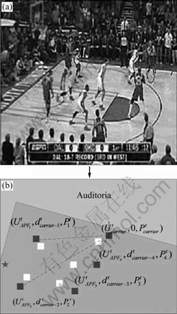
Fig. 3 Example of ball carrier behavior selection

3.3 Prediction of ball receiver

When the output of the RBF predictor is passing ball, the ball receiver can be further predicted. As the ball carrier, he will usually choose the teammate in the most favorable condition within his vision range. In the process of choosing ball receiver, there are two aspects to be considered: more scoring advantage (i.e. higher attractive potential U_goal(x) and lower repulsive potential U_obs(x)), and the distance between the ball carrier and his teammate. The longer distance indicates the higher possibility of passing and catching fault. Hence, the degree of favorable condition of the i-th teammate within the ball carrier’ vision range can be defined as

                            (18)

In Eq. (18),  represents the set of all the teammates within the ball carrier’s vision range at the moment t.  is the APF of the i-th teammate and d_{c, i} is the distance between the i-th teammate and the ball carrier. w₁ and w₂ are the weights of these two factors. According to Eq. (18),  can be computed for each teammate within the ball carrier’s vision range and all of them form a set  Finally, the teammate with the largest  in R_candidate is chosen as the ball receiver.

4 Experiment result and analysis

The effectiveness of the proposed algorithm was verified by using C++ and Matlab hybrid implementation on a PC with Pentium 3.2 GHz processor and 3G RAM. Two experiments were carried out: the first experiment tested the algorithm for determining the vision range of the ball carrier, and the second experiment further proved the effectiveness of the algorithm for predicting the ball carrier’s behavior based on the first one.

4.1 Vision range determination

In order to train the multiclass LogitBoost introduced in Section 2, 4 000 head images are captured as positive samples, making sure that each class has an equal number of images (500). Generally, the head image size varies from 10×10 to 30×30 pixels and they include all kinds of appearance variations such as bold heads, beard faces, light and dark hair and complexion, changes in illumination. After captured, the head images were normalized to a size of 20×20 as training samples of the multiclass LogitBoost. The typical one is displayed in Fig. 4. In addition, 500 head-free images were captured as negative training samples, which were mainly court patches and other body part patches. Figure 5 represents the relation between the ratio of side length of square areas to that of the training samples and recognition ccuracy. It can be concluded that the accuracy peaks when the ratio is 0.28. At the training stage, τ_accuracy for the multiclass LogitBoost was set as 0.99, the learning rate τ_rate was 0.1 and τ_background for head-free image LogitBoost was 0.4. The vision range determination in a real-time basketball match is demonstrated in Fig. 2 and Table 1 gives the experimental result.

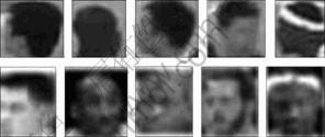
Fig. 3 Typical training examples

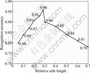
Fig. 4 Relative patch dimension curve

From Table 1, the misclassifications mainly appear in the discrimination of two adjacent head poses due to the low resolution of the head images, noise interference, motion blur and inherent similarity of two adjacent head poses, between which the yaw angle is 45°. The experimental result verifies that the covariance descriptor fusing multiple low level features adjusts well to the condition mentioned above and achieves the promising goal. The average recognition rate of the eight head poses is 83%.

4.2 Behavior prediction of ball carrier

In order to train the RBF predictor in Section 3.2, 654 basketball match videos recorded at 25 fps in NBA (National Basketball Association of USA) regular season and playoffs from 2008 to 2010 were collected as the raw data for the training. The abilities of these teams in the collected videos were at the same level. For each match video, the shooting and tackling results of each player were first recorded and the parameters k_p and k_d were further calculated. Statistically, the initial values of k_p and k_d were set as 10 and 3, respectively. The upper limit θ_d and lower limit η_d of k_d were set as 5 and 1, respectively. The upper limit θ_a and lower limit η_a of k_p were set as 25 and 1, respectively.

After the setting of k_d and k_p for each player, the  corresponding to the moment the ball carrier made the decision (the typical scene is shown in Fig. 3) were automatically computed and further formed a feature vector         and  denoted the actual behavior that the ball carrier chose, in which i is the number of video, j is the number of the ball carrier’s decision-making. After the feature vectors for the collected 654 match videos were computed, a feature vector set S=|i=1, …, 654; j=1, …, n_i} containing 25 363 feature vectors was obtained, in which n_i represents the total number of the ball carrier’s decision-making in the i-th match. Finally, the elements in S were used to train the RBF network.

For the purpose of training the behavior predictor, the learning process of RBF network in our experiment included two stages: unsupervised learning and supervised learning [18]. At the first stage, orthogonal least square (OLS) was adopted to adjust the center of the kernel function; at the second stage, the weight and threshold of the neuron in the output layer were adjusted through least mean square (LMS). After such a learning process, a RBF neural network with 14 input neurons, 68 hidden neurons and 3 output neurons was constructed. In the output layer, 001, 010 and 100 were defined to represent shooting, passing and dribbling, respectively.

In order to determine ω₁ and ω₂ in Eq. (18), the relation between r=ω₁/ω₂ and prediction accuracy was observed, which is revealed in Fig. 6. In Fig. 6, prediction

accuracy is equal to

3N, where   are the prediction accuracies for shooting, passing and dribbling in the i-th match, respectively and N represents the total number of testing videos. It is revealed in Fig. 6 that the prediction accuracy peaks when the ratio is 2.6. As a result, the weights ω₁ and ω₂ were set as 0.72 and 0.28 in our experiments, respectively.

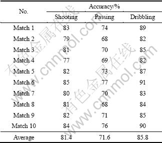
Three examples of typical behavior prediction are shown in Figs. 7-9. In each example, Figs. 7(a), 8(a) and 9(a) are the main interfaces of the system corresponding to the moment that the ball carrier makes the decision; Figs. 7(b), 8(b) and 9(b) are the main interfaces corresponding to the moment that the ball carrier carries out his decision actually. In each figure, the left subwindow shows the video of the basketball match, and the right one shows the player information of the moment shown in the left (the APF information, the distance between the ball carrier and his teammate and the degree of the favorable condition ω), the ball carrier at that moment, the prediction result of the system and the predicted ball receiver. In Fig. 7(a), the system predicted that the ball carrier would pass the ball to teammate A₂. The predictions in Figs. 8(a) and 9(a) are shooting and dribbling, respectively. The figure (b) in each figure proved the correctness of the prediction. The statistic results of ten basketball matches are listed in Table 2.

Table 1 Result of experiment 1

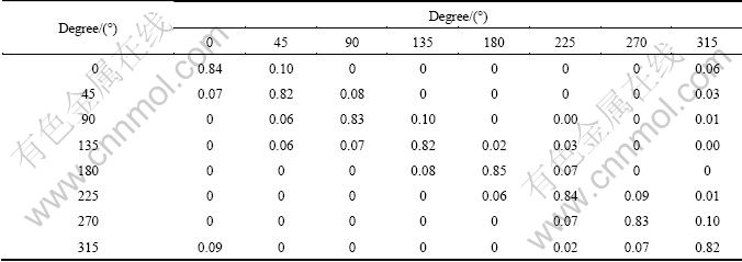
Fig. 6 Relation curve between ratio and accuracy

From Table 2, the average prediction accuracy for both shooting and dribbling is over 80%, which is higher than that of passing. The correct prediction for passing is harder. It requires not only correct prediction for the ball carrier’s passing behavior, but also correct prediction of teammate to which the ball carrier will pass the ball. From the experimental result, the main reasons for wrong prediction are: 1) In basketball matches, the behavior of the ball carrier is impacted by certain given factors as well as some accidental factors, such as change of the player’s physical strength and uncertain injury; 2) Being subjected to tactics and whether the teammates can coordinate smoothly. The reasons mentioned above result in the wrong prediction to some degree.

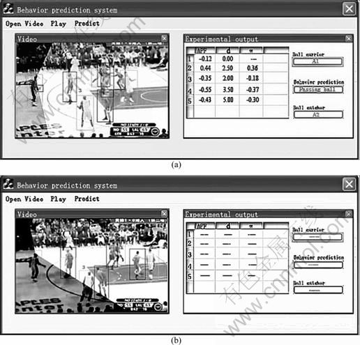
Fig. 7 An example of predicting passing: (a) Predicting passing; (b) Choosing passing

Fig. 8 An example of predicting shooting: (a) Predicting shooting; (b) Choosing shooting

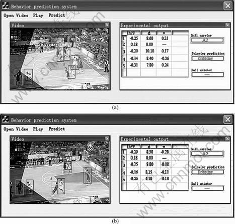
Fig. 9 An example of predicting dribbling: (a) Predicting dribbling; (b) Choosing dribbling

Table 2 Result of Experiment 2

5 Conclusions

1) The vision range of ball carrier is determined by classifying the yaw angle of his head. Aiming at the cluttered background, fast motion of the sportsmen and the low resolution of the head images in the basketball match videos, the covariance descriptor is adopted to fuse multiple visual features of the head region and it can be represented as a point on Riemannian manifold. To determine the vision range of the ball carrier, the covariance descriptor is mapped to the tangent space and the yaw angle classification of his head is completed through the trained multiclass LogitBoost directly in this space.

2) The APF-based information is introduced to describe the court situation of all players within the ball carrier’s vision range, and prediction for the ball carrier’s behavior is completed through the classifier based on RBF neural network.

References

[1] LASHKIA G, OCHIMACHI N, NISHIDA E, HISAMOTO S. A team play analysis support system for soccer games [C]// The 16th International Conference on Vision Interface. Halifax, Canada: IAPR, 2003: 536-541.

[2] LU W L, OKUMA K, LITTLE J J. Tracking and recognizing actions of multiple hockey players using the boosted particle filter [J]. Image and Vision Computing, 2009, 27(1): 189-205.

[3] LI F H, WOODHAM R J. Video analysis of hockey play in selected game situations [J]. Image and Vision Computing, 2009, 27(1): 45-58.

[4] PERSE M, KRISTAN M, PERS J, MUSIC G, VUCKOVIC G. Analysis of multi-agent activity using petri nets [J]. Pattern Recognition, 2010, 43(4): 1491-1501.

[5] DUQUE D, SANTOS H, CORTEZ P. N-ary trees classifier [C]// Proceedings of the 3rd International Conference on Informatics in Control, Automation and Robotics. Setúbal, Portugal: INSTICC, 2006: 256-261.

[6] DUQUE D, SANTOS H, CORTEZ P. Prediction of abnormal behaviors for intelligent video surveillance systems [C]// Proceedings of the 2007 IEEE Symposium on Computational Intelligence and Data Mining. Honolulu, Hawaii, USA: IEEE Press: 2007: 362-367.

[7] COURIER N, HALL D, CROWLEY J L. Estimating face orientation from robust detection of salient facial features [C]// Int Workshop on Visual Observation of Deictic Gestures at POINTING04. Cambridge, United Kingdom: FGnet: 2004: 567-576.

[8] CHEN I, ZHANG L, HU Y, LI M, ZHANG H. Head estimation using fisher manifold learning [C]// Proceeding IEEE International Workshop Analysis and Modeling of Faces and Gestures. Nice, France: IEEE Computer Society: 2003: 203-207.

[9] VALENTI R, LABLACK A, SEBE N, DJERABA C, GEVERS T. Visual gaze estimation by joint head and eye information [C]// 2010 International Conference on Pattern Recognition. Istanbul, Turkey: IEEE Press, 2010: 3870-3874.

[10] TUZEL O, PORIKLI F, MEER P. Pedestrian detection via classification on Riemannian manifolds [J]. IEEE Transactions on Pattern Analysis and Machine Intelligence, 2008, 30(10): 1713-1727.

[11] TUZEL O, PORIKLI F, MEER E. Region covariance: A fast detection and classification [J]. Proceedings of European Computer Vision, 2006, 14(2): 589-600.

[12] FLETCHER P T, JOSHI S. Riemannian geometry for the statistical analysis of diffusion tensor data [J]. Signal Processing, 2007, 87(2): 250-262.

[13] PENNEC X, FILLARD P, AYACHE N. A Riemannian framework for tensor computing [J]. International Journal of Computer Vision, 2006, 66(1): 41-66.

[14] KHATIB O. Real-time obstacle avoidance for manipulators and mobile robots [J]. The International Journal of Robotics Research, 1986, 5(1): 90-98.

[15] XIE Li-juan, XIE Guang-rong, CHEN Huan-wen, LI Xiao-li. Solution to reinforcement learning problems with artificial potential field [J]. Journal of Central South University: Science and Technology, 2008, 15(4): 552-557. (in Chinese)

[16] WANG Y J, TU J. Neural networks control [M]. Beijing: Mechanical Industry Publishing Company, 1998: 68-85. (in Chinese)

[17] BINCHINI M, FRASCONI P, GORI M. Learning without local minima in radial basis function networks [J]. IEEE Transactions on Neural Networks, 1995, 6(3): 749-755.

[18] WEI Hai-kun. The theory and method of neural network structural design [M]. Beijing: National Defense Industry Press, 2005: 62-67. (in Chinese)

(Edited by DENG Lü-xiang)

Foundation item: Project(50808025) supported by the National Natural Science Foundation of China; Project(20090162110057) supported by the Doctoral Fund of Ministry of Education, China

Received date: 2011-06-11; Accepted date: 2011-09-30

Corresponding author: XIA Li-min, Professor, PhD; Tel: +86-731-88830342; E-mail: xlm@mail.csu.edu.cn