Trans. Nonferrous Met. Soc. China 22(2012) s335-s342

Experimental measurement and theoretical prediction of forming limit curve for aluminum alloy 2B06

LI Xiao-qiang, SONG Nan, GUO Gui-qiang

School of Mechanical Engineering and Automation, Beihang University, Beijing 100191, China

Received 28 August 2012; accepted 25 October 2012

Abstract: The main objective of this work was to experimentally and numerically evaluate the forming limit curve (FLC) of aluminum alloy 2B06. The FLC of 2B06 was measured by conducting the hemispherical dome test with specimens of different widths. The theoretical predictions of the FLC of 2B06 were based on the different instability theories and different yield functions. The comparison results show that the influence of the different yield functions can be ignored and the FLCs are basically same utilizing different yield functions based on the specific instability theory. While there is a significant difference among theoretical prediction curves based on three instability theories and the same yield function. The FLC based on SWIFT’s diffuse instability theory is higher than the measured curve. The right part of FLC based on HILL’s localized instability theory is invalid. The theoretical prediction curve based on M-K theory agrees well with the measured FLC. So, the theoretical curves based on M-K theory are effective for predicting the forming limit.

Key words: forming limit curve; M-K theory; theoretical prediction; aluminum alloy 2B06; fracture; yield functions

1 Introduction

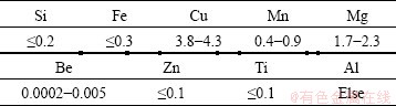
The application of the aluminum alloy has become very extensive in the aerospace field [1]. The aluminum alloys have been widely used in the manufacturing of the aircraft skin because of their excellent performance, such as high specific strength and high specific stiffness. The structural component of aluminum alloy can reduce the 60%-80% of the structural mass of the aircraft [2]. Although the new material is emerging, the application of aluminum alloys on the aircraft will still occupy an irreplaceable role. Aluminum alloy 2B06 is a typical heat-resistant structural material, and belongs to an A1-Cu-Mg system. Aluminum alloy 2B06 is developed based on the aluminum alloy 2A06. The chemical composition is listed in Table 1 [3].

The aluminum alloy 2B06 has a satisfactory performance, such as ductility and fracture toughness by reducing Fe, Si and other impurities. 2B06 can be used on the load-bearing component of the fuselage under continuous working because its softening can be ignored at high temperature. The tensile strength of 2B06 remained approximately constant (the yield strength increases a little) after heating for 1000 h at 175 °C. The deep research of the material’s formability is of significance in sheet metal forming process and finite element simulation [4].

The forming limit is an important performance indicators and process parameters in the field of sheet metal forming, which reflects the largest deformation the sheet can reach before plastic instability in the process. Among a variety of methods evaluating sheet metal formability, the FLC is of the greatest practical significance and is most widely used. The FLC is a very effective tool to evaluate sheet metal formability and solve sheet metal stamping problems [5]. Usually there are two methods to determine the FLC: theoretical calculations and experiments. Theoretical calculation of FLC is based on the specific plastic instability theory including SWIFT’s diffuse instability theories [6], HILL’s localized instability theories [7] and M-K instability theory, using the different yield functions and plastic constitutive equations for theoretical calculation on the forming limit strain. SWIFT’s diffuse instability theory (only valid when biaxial stress state exits) and HILL’s localized instability (no strain rate sensitivity is accounted) theory have some limitations, while MARCINIAK and KUCZYNSKI [8] presented a groove hypothesis from the perspective of material damage, which is the most widely used damage instability theory, known as the M-K theory.

Table 1 Chemical composition of 2B06

The hydro-mechanical deep drawing of aluminum alloy 2B06 and complicated components in aircraft manufacturing were studied by LANG et al [9]. Process design for multi-stage stretch forming of aircraft skin using aluminum alloy 2B06 was studied by HE et al [4]. But the forming limit of 2B06 plate and the influence of the instability theory and yield function have not been reported. In order to characterize the measured FLC, the hemispherical dome test was performed, and the theoretical FLC of the 2B06 based on different instability theories and different yield functions were compared with experimental data in this work. At the same time the analysis results can be used to prove the correctness and accuracy of the theoretical predictions and to establish the theoretical prediction model of FLC for 2B06.

2 Formability test

2.1 Basic formability test

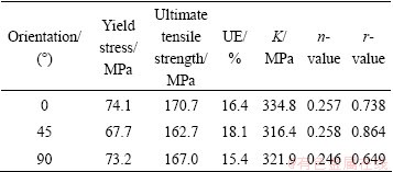
The specimens in three different directions (rolling direction, diagonal and transverse direction) from the 2B06 sheet of 0.8 mm thick were selected in the tensile test according to the standard of GB/T 228—2002 (metallic materials-tensile testing at ambient temperature) [10]. The basic formability parameters are calculated according to the standards of GB/T 5027—1999 (metallic materials-sheet and strip-determination of plastic strain ratio (r-value)) and GB/T 5028—1999 (metallic materials-sheet and strip-determination of strain hardening exponent (n-value)), as listed in Table 2.

Table 2 Basic formability parameters of 2B06

2.2 Forming limit test

The forming limit diagram was obtained by conducting the hemispherical dome test based on the GB/T 15825.8—2008 standard (sheet metal formability and test methods-guidelines for the determination of forming-limit diagrams). Before testing, all the specimens were electro-etched using a grid of circles of 2 mm in diameter. Then the specimens should be placed between the die and blank holder and be pressed by blank holding force at room temperature. The middle part of the test piece will appear bulging deformation and form a convex hull under the action of punch force [11] (shown in Fig. 1). At the same time, the circular grid on the surface of the test piece will be distorted. The principal strains at fracture were estimated by measuring the distortion of the grid as near as possible to the fracture zone, which are used to define the limit principal strains of local surface that sheet metal can withstand. The width of test piece and the lubrication conditions are changed to get a different strain state.

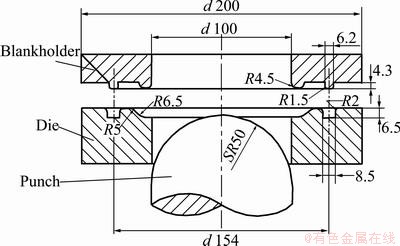
Fig. 1 Rigid punch bulging test (Unit: mm)

The test specimens were prepared by varying the width of blanks from 20 mm to 176 mm (they are 20, 40, 60, 80, 90, 100, 120, 140, 160 and 176 mm), while the horizontal direction (aligned in the transverse direction) is fixed in the length [12,13]. The thickness of the  sample is 0.8 mm. In order to obtain enough test data under different strain states to describe the forming limit curve of the sheet accurately at room temperature, the plates were processed into the sample form shown in Fig. 2.

The tested specimens are shown in Fig. 3. The strain of each test piece was measured and selected according to the standards: 1) Discard the scattered data point from the three points in one group if it is far away from the other two close points. 2) Keep these three points if the three points are gathered together or relatively dispersed in the same coordinate system [14].

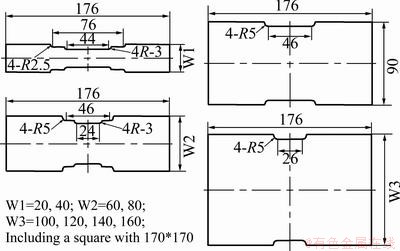
Fig. 2 Geometric dimensions of test piece (Unit: mm)

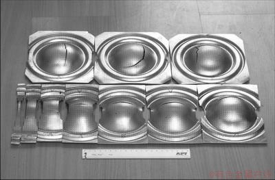
Fig. 3 Tested specimens

3 Theoretical calculation

3.1 Hardening law formulation

The hardening law formulation of 2B06 aluminum alloy can be written as follows [15]:

                                    (1)

The hardening model parameters K and n represent the strength coefficient and strain hardening exponent, respectively. The values of K and n can be got from the fitting data of tensile test based on the constitutive model equation above.

3.2 Yield functions

Different yield functions were selected to calculate the FLC of the 2B06 based on different instability theories: HILL’48 yield function [16], HILL’79 yield function [17], HILL’90 yield function [18], HILL’93 yield function [19], HOSFORD yield function [20], GOTOH [21] yield function and BARLAT-LIAN’89 yield function [22].

1) HILL’48 yield function [16]

In 1948, HILL introduced anisotropy into the yield equation for the first time. He proposed yield function for orthotropic materials following the MISES yield function as a mode and established a reasonable mathematical model to describe the anisotropic plastic flow of sheet metal that laid the foundation for the establishment of the theory of anisotropic plastic deformation.

                (2)

where x, y and z are the orthotropic axes; F, G, H, L, M and N are the independent anisotropic characteristic parameters determined by experiments according to the different materials. A simplified quadratic yield equation facing to a planar isotropic and thick anisotropy material is used in the calculation.

                      (3)

2) HILL’79 yield function [17]

In 1979, HILL proposed a more general yield function:

                    (4)

where σ₁, σ₂ and σ₃ are the principal stresses; f, g, h, a, b and c are independent anisotropy parameters. The value of m can be calculated by

                     (5)

3) HILL’90 yield function [18]

In 1990, HILL introduced the shear stress component into the yield function:

     (6)

                  (7)

where  is the shear stress component, the values of a and b can be calculated from the values of the yield strengths in three directions (0°，45° and 90°).

4) HILL’93 yield function [19]

In 1993, HILL proposed a yield function for specific material ( but ), such as copper sheet.

     (8)

where σ₀ and σ₉₀ are the yield strengths in rolling and transverse directions, respectively; σ_b is the yield strength of the vertex in the hydraulic bulging.

5) HOSFORD yield function [20]

LOGAN and HOSFORD proposed the following yield function for the planar stress state of anisotropic materials in 1979:

            (9)

The value of m in HOSFORD yield function is not adjustable, for body-centered cubic metals, m = 6, for the face-centered cubic metal, m = 8.

6) GOTOH yield function [21]

GOTOH from Japan proposed the yield function in1978:

       (10)

The value of A₁ is 1, and the values of A₂-A₉ can be obtained from the value of r and yield strength.

7) BARLAT-LIAN’89 yield function [22]

In 1989, BARLAT pointed out that HOSFORD yield function can’t handle the situation that the main axes of anisotropy are not aligned with the main stress axes, because HOSFORD yield function does not contain shear stress component. So, BARLAT proposed a yield function considering anisotropism in the planar stress conditions:

    (11)

                            (12)

                 (13)

where σ₀ represents the yield stress of uniaxial tensile test; a, c, h and p are the anisotropy parameters.

3.3 Plastic instability theories

1) SWIFT’s diffuse instability theory [6]

SWIFT held that the external loads in two directions reach the maximum value should be the occurrence condition of the diffuse instability.

                               (14)

But SWIFT’s diffuse instability theory is only valid when biaxial stress state exits under simple loading.

2) HILL’s localized instability theory [7]

HILL presented the localized instability theory under plane stress condition. HILL held that the localized instability occurred along the line of zero strain. The mathematical expression of the instability condition is

                          (15)

But the condition cannot be satisfied because the line of zero strain does not exist under biaxial stretching.

3) M-K instability theory

The core of the M-K theory is the famous assumption of initial inhomogeneity factor. Due to the geometric or physical reasons, there is initial inhomogeneity factor on the direction perpendicular to the direction of maximum principal stress when the biaxial tension exists on the sheet metal surface. That means there is a linear groove before deformation on the sheet surface. The strain concentration will appear and grow in the groove with the degree of deformation increasing. Under this assumption, the localized instability of the sheet is actually caused by the existence of initial surface defects [23].

The theoretical model diagram is shown in Fig. 4, in which part B is uneven deformation zone which is called the groove part and part A is uniform deformation area.

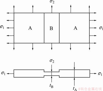
Fig. 4 Mathematical model of M-K theory

The core equations of the M-K theory include [8,23]:

1) The volume of the sheet remains the same along with the sheet deformation:

                          (16)

2) Principal stress in three directions of part A increases in proportion:

                        (17)

The ratio of strains is unchanged through the loading process:

                                (18)

3) The increments of transverse strain (minor strain) are same both in part A and part B:

                           (19)

4) The force equilibrium condition should be satisfied at each moment during deformation (t represents the thickness of the sheet):

                              (20)

5) The initial inhomogeneity factor (f₀):

                                  (21)

3.4 Theoretical prediction of FLC

According to the DRUCKER’s flow theory, the relationship between strain increments:

                      (22)

where

                                 (23)

The stress increment of the sheet metal under external force is

                        (24)

The Eq. (24) can be deduced from the Eq. (1) as:

                              (25)

1) SWIFT’s diffuse instability theory

The condition of the diffuse instability can be deduced from the Eq. (14) as

                               (26)

The limit strains can be deduced from Eqs. (24) and (25) as

                         (27)

2) HILL’s localized instability theory

The limit strains can be deduced from Eq. (15) as

                                 (28)

3) M-K instability theory

When plastic deformation occurs, the strain increases faster in the groove than the strain outside the groove, so the stress state inside and outside the groove are different. Assume that the stress state remains constant in part A because of the stationary linear load, while the load route of part B nonlinearly changes along the different levels of yield surface. The stress state and stress intensity were changed to meet the geometric coordinate conditions and static equilibrium conditions in order to reach the planar strain state, in which the groove deepens () and the material is thought to lose its ability to bear the deformation, and then the localized necking occurs.

Three process parameters were introduced during the calculation process: α, ρ and β. Where α is the ratio of the equivalent stress and major stress (), ρ is the ratio of the minor strain increment and the major strain increment (), β is the ratio of the equivalent strain increment and the major strain increment  ().

The strain increment  of part A is given, with which we can calculate,  and get value of  with the volume conditions:

                          (29)

The strain values change with the increasing of the strain increment as follows:

                                 (30)

Compatibility condition was used to link the two regions A and B with the algorithm:

        (31)

The influence of initial inhomogeneity factor to the prediction of forming limit based on the M-K model cannot be ignored. The determination of initial inhomogeneity factor (f₀) is very complex and error-prone because the initial inhomogeneity factor depends on many factors, including the thickness of the sheet metal, surface quality, grain size and other material properties. The theoretical forming limit curve was defined by adjusting the value of f₀ in practical calculations to make the theoretical FLC₀ (when the minor strain vanishes) close to the experimentally measured FLC₀ in planar strain state. Therefore, the initial inhomogeneity factor is an adjustable parameter in the calculation [24].

The influence of initial inhomogeneity factor to the FLC of 2B06 at room temperature is shown in Fig. 5. Generally, the forming limit curve is higher when the f₀ value is bigger, on the contrary, the forming limit curve is low when the f₀ value is small. The forming limit curve drops down with decreasing of value f₀ till a particular location corresponds to a constant value of f₀.

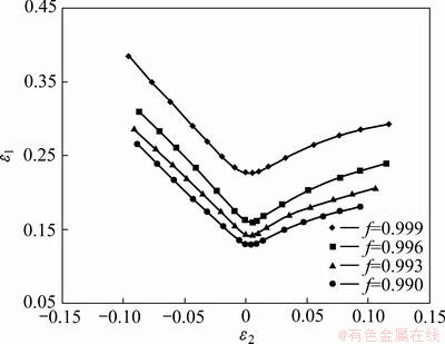
Fig. 5 Influence of initial inhomogeneity factor to FLC

Refer to the forming limit curve shown in the Fig. 7, the theoretical forming limit curve shows a good agreement with the experimentally measured forming limit curve by adjusting the value of f₀ when predicting the FLC at room temperature. Choose 0.99 to be the value of initial inhomogeneity factor (f₀).

4 Theoretical prediction of FLC

4.1 Influence of yield function

Figure 6 is the comparison diagram of the forming limit curves based on HILL’s localized instability theory and different yield functions. Figure 7 is the comparison diagram of the forming limit curves based on SWIFT’s diffuse instability theory and different yield functions. Figure 8 is the comparison diagram of the forming limit curves based on M-K theory and different yield functions. We can draw a conclusion that the FLCs are basically in coincidence respectively in the Figs. 6 and 7. The FLCs are slightly different utilizing different yield functions based on M-K theory.

In summary, the FLCs are basically same utilizing different yield functions based on the specific instability theory.

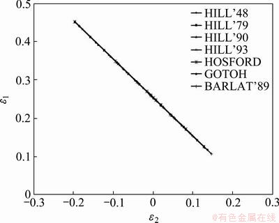
Fig. 6 FLCs based on HILL’s theory and yield functions

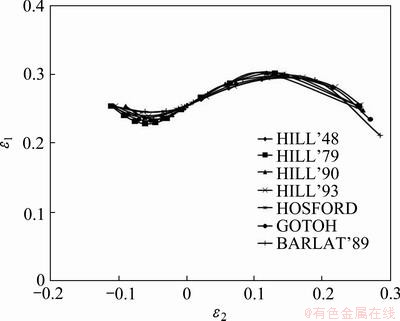
Fig. 7 FLCs based on SWIFT’s theory and yield functions

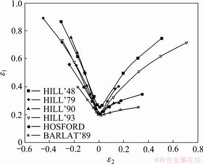
Fig. 8 FLCs based on M-K theory and yield functions

4.2 Influence of instability theory

The theoretical predictions based on the different instability theories and the specific yield function (BARLAT’89) are compared with FLC received from punch bulging test in order to verify the feasibility and correctness of the theoretical predictions (shown in Fig. 9).

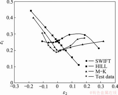
Fig. 9 Comparison diagram of theoretical curves and measured curve

Therefore, we can draw a conclusion that the influence of the different instability theories cannot be ignored because there is significant difference among theoretical prediction curves based on three instability theories. The FLC based on SWIFT’s diffuse instability theory is higher than the measured curve. The right part of FLC based on HILL’s localized instability theory is invalid. While the theoretical prediction curve based on M-K theory agrees well with the measured FLC.

5 Conclusions

1) The basic formability of 2B06 is characterized by uniaxial tension test at room temperature. And the forming limit curve (FLC) of 2B06 is measured by conducting the hemispherical dome test with specimens of different widths.

2) The comparison results of the FLCs show that the influence of the different yield functions can be ignored based on SWIFT’s diffuse instability theory or Hill’s localized instability theory. The FLCs are slightly different utilizing different yield functions based on M-K theory. In summary, the FLCs are basically same utilizing different yield functions based on the specific instability theory.

3) There is a significant difference among theoretical prediction curves based on three instability theories. The FLC based on SWIFT’s diffuse instability theory is higher than the measured curve. The right part of FLC based on Hill’s localized instability theory is invalid. While the theoretical prediction curve based on M-K theory agrees well with the measured FLC.

References

[1] LI X Q, LI D S, ZHOU X B, YANG W J. Plastic anisotropic behavior of a 2806-W aluminum alloy sheet [J]. Journal of Plasticity Engineering, 2008, 15(6): 29-33.

[2] GAO H Z, ZHOU X B. Formability and Numerical Simulation for as-quenched aluminum alloy sheet [J]. Journal of Aeronautical Materials, 2008, 28(5): 27-31.

[3] JIN Y H, HAN D G, LIU X D. Research on smelting and casting process of high pure aluminum alloy 2B06 [J]. Light Alloy Fabrication Technology, 2004, 32(5): 12-15.

[4] HE D H，LI X Q，LI D S, YANG W J. Process design for multi—stage stretch forming of aluminum a11oy aircraft skin [J]. Transactions of Nonferrous Metals Society of China, 2010, 20(6): 1053-1058.

[5] BARATA A R, ABEL D S, PEDRO T, BUTUC M C. Analysis of plastic flow localization under strain paths changes and its coupling with finite element simulation in sheet metal forming [J]. Journal of Materials Processing Technology, 2009, 209(1): 5097-5109.

[6] SWIFT H W. Plastic instability under plane stress [J]. J Mech Phys Solids, 1952, 1(1): 1-18.

[7] HILL R. On discontinuous plastic states with special reference to localized necking in thin sheets [J]. J Mech Phys Solids, 1952, 1(1): 19-31.

[8] MARCINIAK Z, KUCZYNSKI K. Limit strain in the processes of stretch-forming sheet metal [J]. International Journal of Mechanical Sciences, 1967, 9(7): 609-620.

[9] LANG L H, LI T, AN D Y, CHI C L. Investigation into hydro mechanical deep drawing of aluminum alloy—complicated components in aircraft manufacturing [J]. Materials Science and Engineering A, 2009, 499(1-2): 320-324.

[10] KWANSOO C, KANGHWAN A, DONG H Y, KYUNG H C, MIN H S. Formability of TWIP (twinning induced plasticity) automotive sheets [J]. International Journal of Plasticity, 2011, 27(1): 52-81.

[11] WANG Z J, LI Y, LIU J G, ZHANG Y H. Evaluation of forming limit in viscous pressure forming of automotive aluminum alloy 6k21-T4 sheet [J]. Transactions of Nonferrous Metals Society of China, 2007, 17(6): 1169-1174.

[12] ZHOU L, XUE K M, LI P. Determination and application of stress-based forming limit diagram in aluminum tube hydro forming [J]. Transactions of Nonferrous Metals Society of China, 2007, 17(s1): s21-s26.

[13] HUANG G S, ZHANG H, GAO X Y, SONG B, ZHANG L. Forming limit of textured AZ31B magnesium alloy sheet at different temperatures [J]. Transactions of Nonferrous Metals Society of China, 2011, 21(4): 836-843.

[14] HE M, LI F G, WANG Z G. Forming limit stress diagram prediction of aluminum alloy 5052 based on GTN model parameters determined by in situ tensile test [J]. Chinese Journal of Aeronautics, 2011, 24(3): 378-386.

[15] MARILENA C, BUTUC, CRISTIAN T, BARLAT, GRACIO J J. Analysis of sheet metal formability through isotropic and kinematic hardening models [J]. European Journal of Mechanics A/Solids, 2011, 30(4): 532-546.

[16] HILL R. A theory of the yielding and plastic flow of anisotropic metals [J]. Proceedings of Royal Society of London, 1948, 193(1033): 281-297.

[17] HILL R, HAVNER K S. Perspectives in the mechanics of elastoplastic crystals [J]. Journal of the Mechanics and Physics of Solids, 1982, 30(1-2): 5-22.

[18] HILL R. Constitutive modeling of orthotropic plasticity in sheet metals [J]. Journal of the Mechanics and Physics of Solids, 1990, 38(3): 405-417.

[19] SIGUANG X，KLAUS J. Prediction of forming limit curves of sheet metals using Hill’s 1993 user-friendly yield criterion of anisotropic materials [J]. Int J Mach Sci, 1998, 40(9): 913-925.

[20] HOSFORD W F. On yield loci of anisotropic cubic metals [C]// Proceedings of the 7th North. American Metalworking Research Conference, Ann Arbor, USA: University of Michigan, 1979: 191-197.

[21] GOTOH M, F. A finite element analysis of rigid-plastic deformation of the flange in a deep drawing process based on a fourth-degree yield function [J]. International Journal of Mechanical Sciences, 1978, 20(7): 423-435.

[22] BARLAT F, LIAN K. Plastic behavior and stretchability of sheet metals. Part I: A yield function for orthotropic sheets under plane stress conditions [J]. International Journal of Plasticity, 1989, 5(1): 51-66.

[23] MORTEZA N, DANIEL E G. Prediction of sheet forming limits with Marciniak and Kuczynski analysis using combined isotropic- nonlinear kinematic hardening [J]. International Journal of Mechanical Sciences, 2011, 53(2): 145-153.

[24] SERENELLI M J, BERTINETTI M A, SIGNORELLI J W. Investigation of the dislocation slip assumption on formability of BCC sheet metals [J]. International Journal of Mechanical Sciences, 2010, 52(12): 1723-1734.

2B06铝合金板成形极限图的实验测定与理论预测

李小强，宋  楠，郭贵强

北京航空航天大学 机械工程及自动化学院，北京 100191

摘  要：通过实验确定和理论计算得到2B06铝合金板的成形极限图(FLC)。在凸模胀形实验中通过改变试件的宽度得到完整的FLC。理论预测的FLC是基于不同失稳理论和不同的屈服准则计算得到的。通过对比可知，基于同一失稳理论和不同屈服准则的预测曲线区别不大，所以不同屈服准则对理论预测的影响并不大。而基于不同失稳理论的理论曲线之间差距很大。基于SWIFT分散性失稳理论的FLC曲线比试验测定的曲线要高。基于HILL集中性失稳理论的FLC右半边曲线不可用。应用M-K理论的FLC预测曲线与试验结果最为接近，所以M-K可以作为理论计算预测成形极限图的有效方式。

关键词：成形极限曲线；M-K理论；理论预测；2B06铝合金；断裂；屈服准则

(Edited by DENG -xiang)

Foundation item: Project (50905008) supported by the National Natural Science Foundation of China; Project (513180102) supported by the National Defense Pre-research Program of China; Project (SAMC12JS-15-008) supported by Foundation of National Engineering and Research Center for Commercial Aircraft Manufacturing, China

Corresponding author: LI Xiao-qiang; Tel: +86-10-82316584; E-mail: lixiaoqiang@buaa.edu.cn

DOI: 10.1016/S1003-6326(12)61728-2